7 Epidemic models—Practical 2

Andrew Conlan (ajkc2@cam.ac.uk), Sophie Ip, Ellen Brooks Pollock (ellen.brooks-pollock@bristol.ac.uk)

7.1 Outline

In this practical we will:

• Code and run a model with vaccination.
• Investigate the critical vaccination threshold.
• Code and run a two-population model and investigate targeted vaccination.

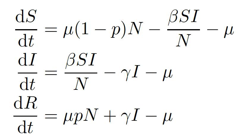
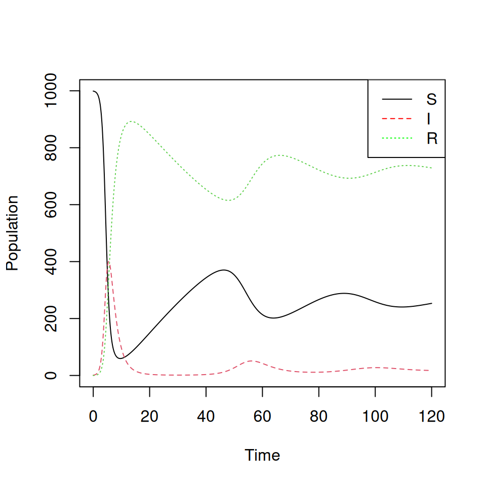
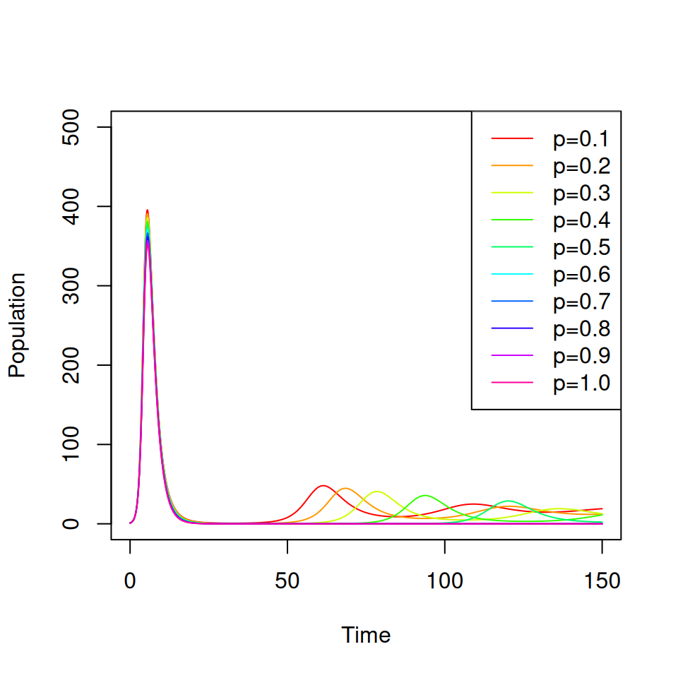
7.2 Vaccination at birth

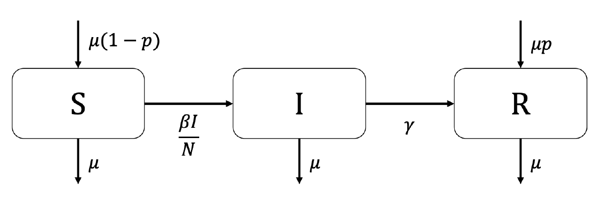
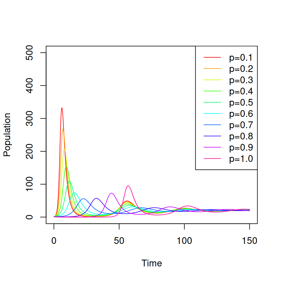
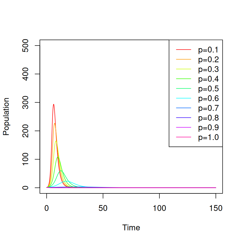
Consider a vaccine that confers complete protection against infection for life that is administered at birth. You will need to adapt your SIR model from practical 1 to include births, deaths and a permanent vaccination campaign where a proportion \(p \leq 1\) of all newborns are immunized.

Task

Sketch out the model. Hint: You don’t necessarily have to include a vaccinated compartment as you could include vaccinated people in the ‘recovered’ compartment.

Solution

Task

Write down the modified equations.

Solution

Task

Adapt your SIR model with births and deaths to include vaccination and run the model with parameters \(\beta = 2\), \(\gamma = 0.5\), \(\mu = 1/70\), \(p=0\) and initial conditions \(S(t = 0) = 999\), \(I(t = 0) = 1\) and \(R(t = 0) = 0\).

Solution

library(deSolve)

SIR.dyn <- function(t,var,par) {
    S <- var[1]
    I <- var[2]
    R <- var[3]
    N <- S+I+R
    beta <- par[1]
    gamma <- par[2]
    mu <- par[3]
    p <- par[4]
    
    dS <- (1-p)*mu*N - beta*S*I/N - mu*S
    dI <- beta*S*I/N - gamma*I - mu*I
    dR <- gamma*I - mu*R + p*mu*N
    return(list(c(dS,dI,dR)))
}

SIR.par<-c(beta=2,gamma=0.5,mu=1/70.0,p=0)
SIR.init<-c(S=999,I=1,R=0)
SIR.t<-seq(0,120,0.1)
  
det.sol <- lsoda(SIR.init,SIR.t,SIR.dyn,SIR.par)

matplot(det.sol[,1],det.sol[,2:4],type='l',xlab='Time',ylab='Population')
legend('topright',c('S','I','R'),col=c('black','red','green'),lty=c(1,2,3))

Task

What’s the critical vaccination threshold for these parameters, \(p_{vac}\)?

Solution

\(p_{vac} = 1 - \frac{1}{R_{0}} = 1 - \frac{\gamma + \mu}{\beta} = 26/35 \simeq 0.75\)

Task

Investigate increasing the proportion of vaccinated newborns from 0 to 1. What happens to the number of infected individuals when p crosses the critical vaccination threshold?

Solution

# Values of vaccination coverage to try
p_vals = seq(0.1,1.0,0.1)
# Color palette for plotting
col_vals = rainbow(length(p_vals))

# Make an empty plot
plot(0,xlim=c(0,150),ylim=c(0,500),pch=' ',xlab='Time',ylab='Population')

# Initial conditions and time points same for each solution
SIR.init<-c(S=999,I=1,R=0)
SIR.t<-seq(0,150,0.1)

for(i in 1:length(p_vals)) {
    # Change vaccination coverage
    SIR.par<-c(beta=2,gamma=0.5,mu=1/70.0,p=p_vals[i])
      
    det.sol <- lsoda(SIR.init,SIR.t,SIR.dyn,SIR.par)
    
    # plot I curve only
    
    lines(SIR.t,det.sol[,3],col=col_vals[i])
}

legend('topright',c('p=0.1',
                    'p=0.2',
                    'p=0.3',
                    'p=0.4',
                    'p=0.5',
                    'p=0.6',
                    'p=0.7',
                    'p=0.8',
                    'p=0.9',
                    'p=1.0'),col=col_vals,lty=1)

Question

Why do you still get an initial epidemic?

Answer

We can see that for \(p < p_{vac}\), we have a second outbreak following the initial first outbreak. This does not occur if \(p > p_{vac}\). We still get an initial epidemic in all cases because we start with an entirely susceptible population. Since we only vaccinate individuals as they are born, it takes some time for the total proportion of population vaccinated to be high enough to ensure herd immunity.

Task

Plot a horizontal line to indicate \(1/R_0\). Notice what happens to the number of susceptible when \(p = 0.75\). What about when \(p = 0.7\)?

Solution

# Values of vaccination coverage to try
p_vals = seq(0.1,1.0,0.1)
# Color palette for plotting
col_vals = rainbow(length(p_vals))

# Make an empty plot
plot(0,xlim=c(0,150),ylim=c(0,1000),pch=' ',xlab='Time',ylab='Population')

# Add herd immunity threshold

abline(h=(1-26/35)*1000,col='black',lwd=2)

# Initial conditions and time points same for each solution
SIR.init<-c(S=999,I=1,R=0)
SIR.t<-seq(0,150,0.1)

for(i in 1:length(p_vals)) {
    # Change vaccination coverage
    SIR.par<-c(beta=2,gamma=0.5,mu=1/70.0,p=p_vals[i])
      
    det.sol <- lsoda(SIR.init,SIR.t,SIR.dyn,SIR.par)
    
    # plot S curve only
    
    lines(SIR.t,det.sol[,2],col=col_vals[i])
}

legend('topright',c('p=0.1',
                    'p=0.2',
                    'p=0.3',
                    'p=0.4',
                    'p=0.5',
                    'p=0.6',
                    'p=0.7',
                    'p=0.8',
                    'p=0.9',
                    'p=1.0'),col=col_vals,lty=1)

In all cases except \(p = 1\), we tend towards the steady state at \(\frac{1}{R_{0}}\) (shown in black). If \(p < p_{vac}\), the proportion of susceptibles increases after the initial peak and overshoots \(\frac{1}{R_{0}}\) before fluctuating and settling to the steady state; otherwise the number of susceptibles slowly increases to the steady state.

Task

Modify your model to include a one-off vaccination campaign at the start so that there is no initial epidemic.

Solution

First consider one-off campaign on it’s own without vaccination at birth.

# Values of vaccination coverage to try
p_vals = seq(0.1,1.0,0.1)
# Color palette for plotting
col_vals = rainbow(length(p_vals))
# Vaccination at birth now 0
SIR.par<-c(beta=2,gamma=0.5,mu=1/70.0,p=0.0)
  
# Make an empty plot
plot(0,xlim=c(0,150),ylim=c(0,500),pch=' ',xlab='Time',ylab='Population')

# Time points same for each solution

SIR.t<-seq(0,150,0.1)

for(i in 1:length(p_vals)) {
    # Now model one-off vaccination campaign at start by modifying the initial conditions
    SIR.init<-c(S=(999)*(1-p_vals[i]),I=1,R=(999)*(p_vals[i]))  
      
    det.sol <- lsoda(SIR.init,SIR.t,SIR.dyn,SIR.par)
    
    # plot I curve only
    lines(SIR.t,det.sol[,3],col=col_vals[i])
}

legend('topright',c('p=0.1',
                    'p=0.2',
                    'p=0.3',
                    'p=0.4',
                    'p=0.5',
                    'p=0.6',
                    'p=0.7',
                    'p=0.8',
                    'p=0.9',
                    'p=1.0'),col=col_vals,lty=1)

A single one off campaign can delay - but not prevent an epidemic. Even for \(p>0.75\), there will still be an smaller outbreak once enough births have accumulated to bring the number of susceptibles above the herd immunity threshold.

If we now consider a one-off campaign in addition to vaccination at birth at 75%:

# Values of vaccination coverage to try
p_vals = seq(0.1,1.0,0.1)
# Color palette for plotting
col_vals = rainbow(length(p_vals))
# Vaccination at birth now 0.75
SIR.par<-c(beta=2,gamma=0.5,mu=1/70.0,p=0.75)
  
# Make an empty plot
plot(0,xlim=c(0,150),ylim=c(0,500),pch=' ',xlab='Time',ylab='Population')

# Time points same for each solution

SIR.t<-seq(0,150,0.1)

for(i in 1:length(p_vals)) {
    # Now model one-off vaccination campaign at start by modifying the initial conditions
    SIR.init<-c(S=(999)*(1-p_vals[i]),I=1,R=(999)*(p_vals[i]))  
      
    det.sol <- lsoda(SIR.init,SIR.t,SIR.dyn,SIR.par)
    
    # plot I curve only
    
    lines(SIR.t,det.sol[,3],col=col_vals[i])
}

legend('topright',c('p=0.1',
                    'p=0.2',
                    'p=0.3',
                    'p=0.4',
                    'p=0.5',
                    'p=0.6',
                    'p=0.7',
                    'p=0.8',
                    'p=0.9',
                    'p=1.0'),col=col_vals,lty=1)

Now we can see that increasing \(p\) for an initial campaign not only decreases the size of the initial outbreak, but for \(p > p_{vac}\) for the initial campaign, there is now no outbreak.

Question

What does this tell you about vaccination at birth programmes used in isolation?

Answer

This suggests that birth programmes used in isolation are insufficient to prevent outbreaks; we also need a sufficiently large proportion of the population immune to begin with.

7.3 Targeted Vaccination

Now we will consider vaccination in a population with two age groups. We assume that the epidemic dynamics are much faster than demographic changes, so the impact of births and deaths is negligible. Firstly, code up a two-population model. You can base it on the code from the earlier SIR practical.

# This proposed version uses some helpful features of the R language to simplify the code:
# "with" allows us to bring named members of a vector into the local namespace
# here we use to avoid having to specifically rename the elements of par
# We use the matrix/vector functionality to avoid writing down individual equations for 
# each group. We don't need to do this it would just be longer to write out each equation in 
# turn. You should try this as an excercise and check your new function gives the same dynamics!

TwoPopSIR <- function(t,states,par) {

  with(as.list(c(states, par)), {
  
        pops<-matrix(states[1:(npops*nstates)],
        nrow=nstates,ncol=npops,byrow=T)
        
        S=pops[1,]
        I=pops[2,]
        R=pops[3,]
        
        N=colSums(pops)
        
        newinfections = colSums(beta*(I/N) %*% t(S))
        dS <- -newinfections
        dI <- newinfections - gamma*I
        dR <- gamma*I
        return(list(c(dS,dI,dR)))
    })
}

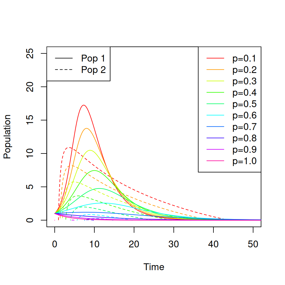
Run the model with initial conditions init <- c(49,50,1,0,0,0) and parameters \(\gamma = \frac{1}{4}\) and \(\beta = \left( \begin{matrix} 1 & 0.1 \\ 0.1 & 0.5 \end{matrix} \right)\).

# states are recorded in order (S1,S2,I1,I2,R1,R2)
# so we have 1 infected in patch 1 for initial condition, 50 individuals in both patches

TwoPop.init<-c(49,50,1,0,0,0)

# Note we have been lazy here and have written the function
# to use the "beta" matrix from the global workspace. This is bad programming form
# but again avoids messing about converting the matrix to and from vectors...

beta = matrix(c(1,0.1,0.1,0.5),2,2)

# As transmission parameters coded in beta above, one other parameter (named for use with with above). Also need number of states and patches (npops) to convert between vector/matrix
TwoPop.par<-c(gamma=1/4.0,nstates=3,npops=2)

TwoPop.t<-seq(0,120,0.1)

TwoPop.sol <- lsoda(TwoPop.init,TwoPop.t,TwoPopSIR,TwoPop.par)

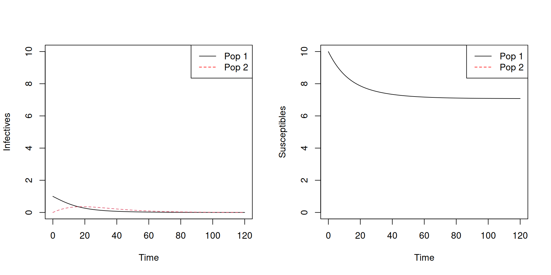
matplot(TwoPop.sol[,1],TwoPop.sol[,c(4,5)],type='l',xlab='Time',ylab='Infectives')
legend('topright',c('Pop 1','Pop 2'),col=c('black','red'),lty=c(1,2))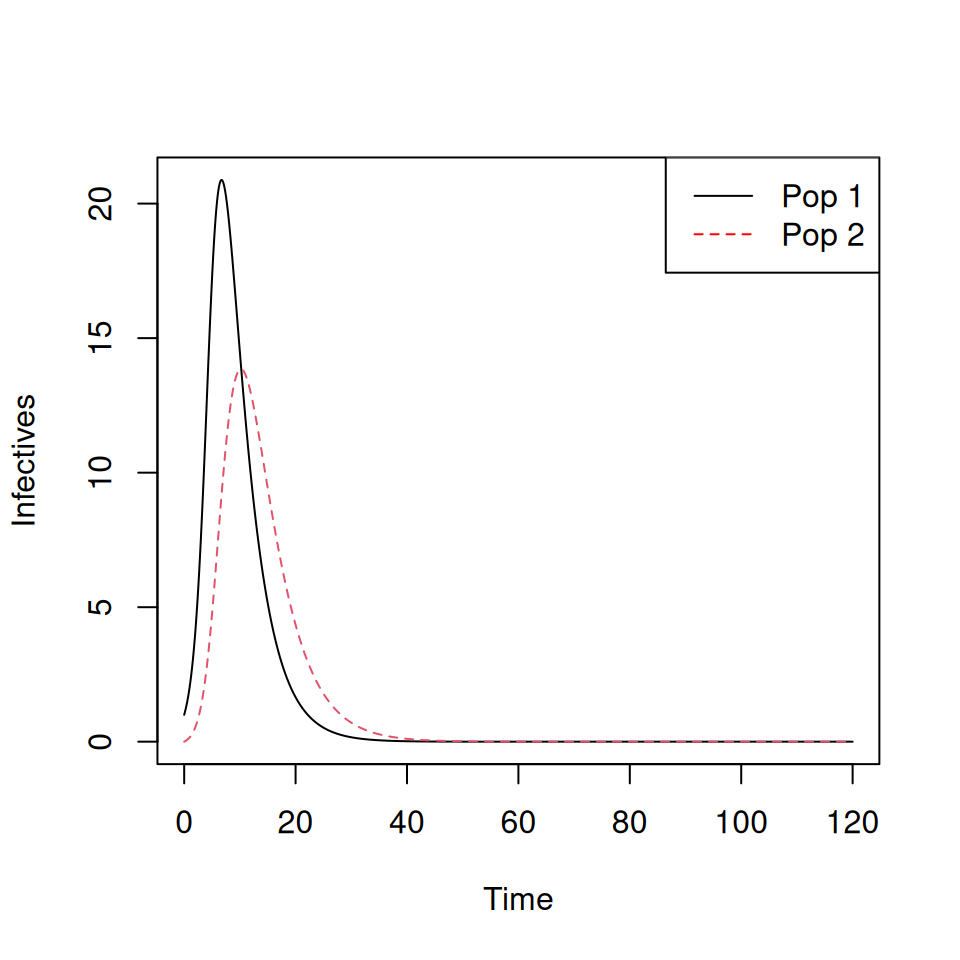

matplot(TwoPop.sol[,1],TwoPop.sol[,c(2,3)],type='l',xlab='Time',ylab='Susceptibles')
legend('topright',c('Pop 1','Pop 2'),col=c('black','red'),lty=c(1,2))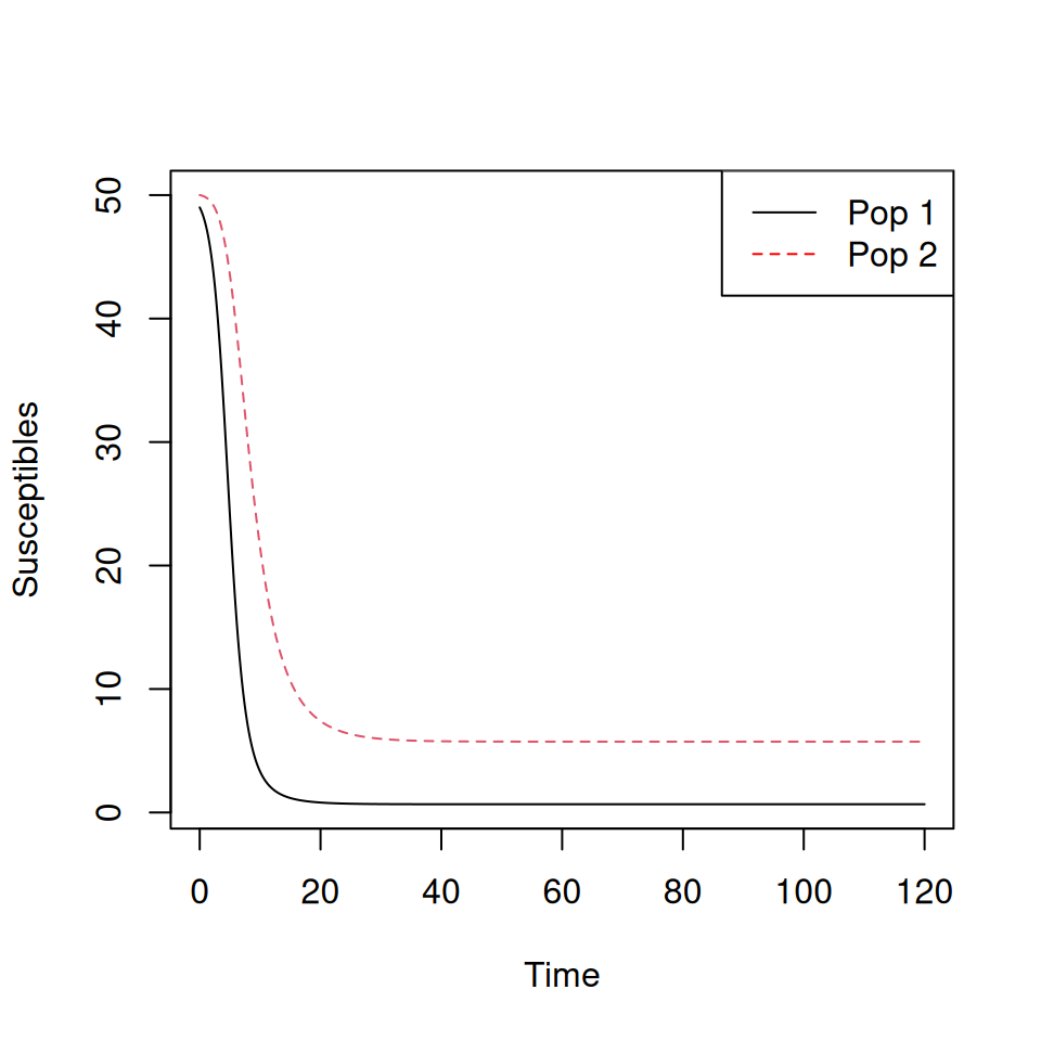

Note that the epidemic peak occurs later, and is lower, for group 2.

Task

Write down the next generation matrix for these parameters and calculate \(R_{0}\).

Solution

\(K = \frac{1}{\gamma} \beta = \left( \begin{matrix} 4 & 0.4 \\ 0.4 & 2 \end{matrix} \right)\)

Task

What is the critical vaccination threshold for this disease?

Solution

Using the formula for \(R_{0}\) from the lectures:

\(R_{0} = \frac{4 + 2 + \sqrt{(4+2)^2 - 4(4 \times 2 - 0.4^2) }}{2} \simeq 4.08\)

The critical vaccination threshold is

# Next Generation Matrix and R0

ngm = (4.0)*matrix(c(1,0.1,0.1,0.5),byrow=T,nrow=2) 

R0 = max(eigen(ngm)$values)

p_critical = 1 - 1/R0

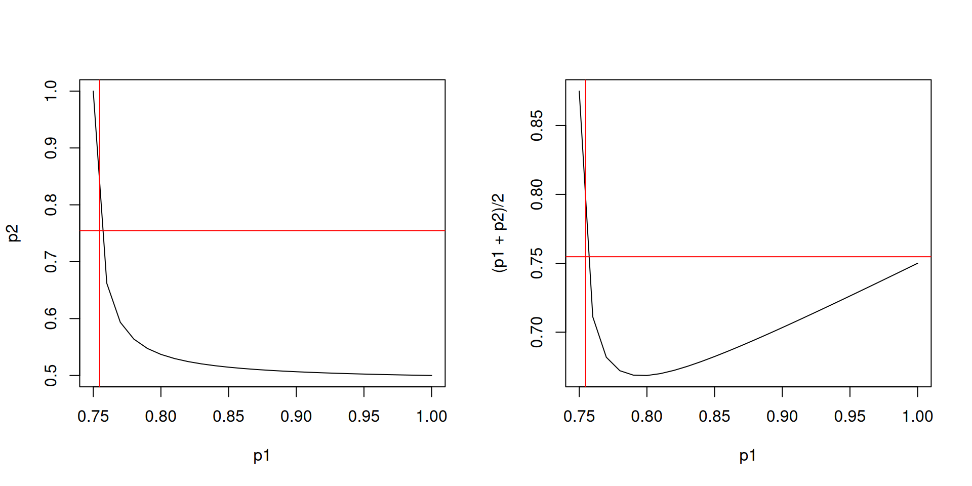
Let’s assume that a proportion \(p_1\) of group 1 and a proportion \(p_2\) of group 2 are vaccinated at the start of the model. The initial conditions are:

p1=0.8
p2=0.8
init <- c(49*(1-p1),50*(1-p2),1,0,49*p1,50*p2)

Task

By changing the initial conditions, explore the dynamics with random vaccination, where \(p_1 = p_2\).

Solution

# Values of vaccination coverage to try
p_vals = seq(0.1,1.0,0.1)
# Color palette for plotting
col_vals = rainbow(length(p_vals))

# Make an empty plot
plot(0,xlim=c(0,50),ylim=c(0,25),pch=' ',xlab='Time',ylab='Population')

for(i in 1:length(p_vals)) {
    # Now model one-off vaccination campaign at start by modifying the initial conditions
    init <- c(49*(1-p_vals[i]),50*(1-p_vals[i]),1,0,49*p_vals[i],50*p_vals[i]) 
      
    TwoPop.sol <- lsoda(init,TwoPop.t,TwoPopSIR,TwoPop.par)
    
    # plot I curve only
    
    lines(TwoPop.sol[,1],TwoPop.sol[,4],col=col_vals[i],lty=1)
    lines(TwoPop.sol[,2],TwoPop.sol[,5],col=col_vals[i],lty=2)
}

legend('topright',c('p=0.1',
                    'p=0.2',
                    'p=0.3',
                    'p=0.4',
                    'p=0.5',
                    'p=0.6',
                    'p=0.7',
                    'p=0.8',
                    'p=0.9',
                    'p=1.0'),col=col_vals,lty=1)

legend('topleft',c('Pop 1','Pop 2'),col='black',lty=c(1,2))

Task

Using the formula from the lecture, plot the total proportion of the population that needs to be vaccinated to prevent an epidemic \(\frac{(p1 + p2)}{2}\) for different values of \(p_{1}\).

Solution

# Critical proportion (p2) that needs to be vaccinated given a value of p1
# Using equation from lectures

a = ngm[1,1];b = ngm[1,2]; c = ngm[2,1]; d = ngm[2,2]

# p1 must be greater than 1 - 1/a
p1 = seq(1-1/a,1,0.01)

p2 = 1 - ((1 - a*(1-p1))/(d - (a*d - b*c)*(1-p1)))

par(mfrow=c(1,2))

plot(p1,p2,type='l')
abline(v=p_critical,col='red')
abline(h=p_critical,col='red')
plot(p1,(p1+p2)/2,type='l')
abline(v=p_critical,col='red')
abline(h=p_critical,col='red')
par(mfrow=c(1,1))

We can read off the minimum possible value of p off our graph. This gives \(p \simeq 0.668\), \(p_{1} \simeq 0.796\) and \(p_{2} \simeq 0.541\). Overall, this is a lower level of vaccination than random vaccination, so may be more efficient. The optimal vaccination scenario below, not that although the number of infectives in the second population initially increase it never crosses 1.

p1=0.796
p2=0.541
Optimal.init<- c(49*(1-p1),50*(1-p2),1,0,49*p1,50*p2)

TwoPop.t<-seq(0,120,0.1)
# Note, at optimal coverage I[2] initially increases, but never crosses 1...

TwoPop.sol <- lsoda(Optimal.init,TwoPop.t,TwoPopSIR,TwoPop.par)

par(mfrow=c(1,2))
matplot(TwoPop.sol[,1],TwoPop.sol[,c(4,5)],type='l',xlab='Time',ylab='Infectives',ylim=c(0,10))
legend('topright',c('Pop 1','Pop 2'),col=c('black','red'),lty=c(1,2))
matplot(TwoPop.sol[,1],TwoPop.sol[,c(2,3)],type='l',xlab='Time',ylab='Susceptibles',ylim=c(0,10))
legend('topright',c('Pop 1','Pop 2'),col=c('black','red'),lty=c(1,2))
par(mfrow=c(1,1))