3 Programming—Practical 1

Nik Cunniffe (njc1001@cam.ac.uk)

3.1 Getting started

Start a new RStudio session, set your current working directory, open a new R Script and save this (blank) script to a file with an appropriate name.

Use this script file to edit and keep copies of the code you write in this practical: you may find it useful be able to look back later.

3.2 Predicting the behaviour of for loops

We will use R to generate some data in the form of vectors and use these data to form some looping constructs. Predicting what code will do and testing your predictions by running the code should help cement your understanding of for loops.

Type the following code into your script. Remember that code after # is a comment and will be ignored by the R interpreter (you do not have to type these comments in for yourself, but you might want to if you think you will need to refer to them later).

a <- 1:10           # Assign the integers 1 to 10 in order to the vector a
print(a)            # Print a to the screen
b <- sample(a)      # Set b to be a with elements shuffled into random order
print(b)            # Print b to the screen

Run the code a few times either by sourcing it or by highlighting it in the script then pressing the run button in RStudio.

You should note that:

• The first line creates a new vector a with the elements 1 to 10 in order.
• The second line prints the vector a to the screen.
• The third line uses a built-in R function to sample (all of) the elements of the vector a without replacement (i.e. to permute the elements into a random order), and assigns the result to the vector b.
• The fourth line prints the vector b.

You should also note that the code gives a different result each time you run it, since repeating the sample command leads to b being set to a new permutation of a.

Task

Write down what you expect the output of the following code to be before verifying your answer by entering the code into your script and running it.

for (i in 1:10) {
    print(paste(i, a[i]))
}

Solution

Prints numbers in order.

## [1] "1 1"
## [1] "2 2"
## [1] "3 3"
## [1] "4 4"
## [1] "5 5"
## [1] "6 6"
## [1] "7 7"
## [1] "8 8"
## [1] "9 9"
## [1] "10 10"

Task

Write down what you expect the output of the following code to be before verifying your answer by entering the code into your script and running it.

for (i in 10:1) {
    print(paste(i, b[i]))
}

Solution

Prints numbers in reverse order according to whatever is in sample b.

## [1] "10 5"
## [1] "9 9"
## [1] "8 10"
## [1] "7 2"
## [1] "6 7"
## [1] "5 1"
## [1] "4 3"
## [1] "3 4"
## [1] "2 6"
## [1] "1 8"

Task

Write down what you expect the output of the following code to be before verifying your answer by entering the code into your script and running it.

for (i in a) {
    print(paste(i, b[i]))
}

Solution

Prints numbers in forward order according to whatever is in vector b.

## [1] "1 8"
## [1] "2 6"
## [1] "3 4"
## [1] "4 3"
## [1] "5 1"
## [1] "6 7"
## [1] "7 2"
## [1] "8 10"
## [1] "9 9"
## [1] "10 5"

Task

Write down what you expect the output of the following code to be before verifying your answer by entering the code into your script and running it.

for (i in sample(a)) {
    print(paste(i, b[i]))
}

Solution

Prints numbers in a random order from whatever is in vector b.

## [1] "9 9"
## [1] "6 7"
## [1] "10 5"
## [1] "2 6"
## [1] "8 10"
## [1] "1 8"
## [1] "7 2"
## [1] "3 4"
## [1] "4 3"
## [1] "5 1"

3.3 Writing a for loop

Adapt the code from the lecture to use a for loop to do the following:

Task

Print the 12 times table using a for loop, i.e. produce output of the form

• 1 times 12 is 12
• 2 times 12 is 24
• \(\dots\)
• 12 times 12 is 144

Solution

for (i in 1:12) {
    result <- i * 12
    print(paste(i, "times 12 is", result))
}

## [1] "1 times 12 is 12"
## [1] "2 times 12 is 24"
## [1] "3 times 12 is 36"
## [1] "4 times 12 is 48"
## [1] "5 times 12 is 60"
## [1] "6 times 12 is 72"
## [1] "7 times 12 is 84"
## [1] "8 times 12 is 96"
## [1] "9 times 12 is 108"
## [1] "10 times 12 is 120"
## [1] "11 times 12 is 132"
## [1] "12 times 12 is 144"

3.4 Writing a while loop

Repeat the previous task using a while loop.

Task

Print the 12 times table using a while loop, i.e. produce output of the form

• 1 times 12 is 12
• 2 times 12 is 24
• \(\dots\)
• 12 times 12 is 144

Solution

i <- 1
while(i <= 12) {
  result <- i * 12
  print(paste(i, "times 12 is", result))
  i <- i + 1
}

## [1] "1 times 12 is 12"
## [1] "2 times 12 is 24"
## [1] "3 times 12 is 36"
## [1] "4 times 12 is 48"
## [1] "5 times 12 is 60"
## [1] "6 times 12 is 72"
## [1] "7 times 12 is 84"
## [1] "8 times 12 is 96"
## [1] "9 times 12 is 108"
## [1] "10 times 12 is 120"
## [1] "11 times 12 is 132"
## [1] "12 times 12 is 144"

3.5 Using loops to do more complex calculations

3.5.1 A loop for which the number of iterations is known in advance

Enter the following code to your script and check you understand the output.

p <- 4
print(2^p)
p <- 5
print(p^3)

Now write code to answer the following question.

Task

What is the sum of the first 15 powers of 2 (i.e. \(2^1 + 2^2 + \dots 2^{15}\))?

Solution

runningSum <- 0
for(i in 1:15) {
  runningSum <- runningSum + 2^i
}
print(paste("Sum is", runningSum))

## [1] "Sum is 65534"

Note you can do the above more efficiently using vectorised operators, e.g. sum(2^(1:15)).

3.5.2 A loop for which the number of iterations is not known in advance

Write code to answer the following question.

Task

What is the smallest power of 2 that is greater than 1,000,000?

Solution

thisIDX <- 1
thisPower <- 2^thisIDX
while(thisPower<1000000) {
  thisIDX <- thisIDX + 1
  thisPower <- 2^thisIDX
}
print(paste("2^",thisIDX,"=",thisPower,sep=""))

## [1] "2^20=1048576"

3.6 Writing simple functions

Type the following code into your script and run it. Before you run it, think about whether you expect any output.

sayHello <- function() {
    print("Hello")
}

Type the following at the command prompt, but before you do so, predict what will happen.

sayHello()

Now type the following code into your script.

sayHelloWithArg <- function(whoTo) {
    print(paste("Hello", whoTo))
}

Task

Now type each of the following instructions into the command prompt. Before typing each line, predict what will happen.

sayHelloWithArg()
sayHelloWithArg 
sayHelloWithArg("nik")
sayHello("nik")
sayHelloWithArg(nik) 
sayHelloWithArg(whoto="nik") 
sayHelloWithArg(whoTo="nik")

Solution

sayHelloWithArg()       # error, since not passed argument

## Error in sayHelloWithArg(): argument "whoTo" is missing, with no default

# echos function's code to screen (happens in general if 
# type function's name without brackets)
sayHelloWithArg

## function(whoTo) {
##     print(paste("Hello", whoTo))
## }

sayHelloWithArg("nik")  # works as expected

## [1] "Hello nik"

sayHello("nik")         # error, since too many arguments for the simpler function

## Error in sayHello("nik"): unused argument ("nik")

sayHelloWithArg(nik)    # error, since variable nik is not defined

## Error in eval(expr, envir, enclos): object 'nik' not found

sayHelloWithArg(whoto="nik") # error, since argument names are case sensitive

## Error in sayHelloWithArg(whoto = "nik"): unused argument (whoto = "nik")

sayHelloWithArg(whoTo="nik") # works as expected

## [1] "Hello nik"

3.7 Predicting the behaviour of a function

For now, do not type in the following code, but instead just read it.

cat <- 2
canary <- 4
buster <- function(cat, canary) { 
  cat <- cat*2 
  canary <- canary*3
  return(cat + canary) 
}
ghost <- buster(canary, -cat)

Task

Think carefully about what you expect the values of cat, canary and ghost to be after this code is executed and write down your answer. Now execute the code and test your prediction.

Solution

The line ghost <- buster(canary, -cat) sets ghost to be 2, but leaves cat and canary unchanged.

3.8 Return values from functions

The code in the box below does the following.

• Defines a function mySum that returns the sum of a vector.
• Creates a vector x containing 100 uniform random numbers between 0 and 1.
• Finds their sum using mySum.
• Finds their sum using the built-in R function sum.
• Prints out a comparison of the two values.

Type the code into your script and make sure you are happy with how it works.

mySum <- function(toSum) { # my function to sum elements of a vector
  retVal <- 0
  for(i in 1:length(toSum)) { 
    retVal <- retVal + toSum[i]  
  } 
  return(retVal)
} 

a <- runif(100)     # generate 100 uniform random numbers 
myWay <- mySum(a)   # calculate sum using our mySum() function
rWay <- sum(a)      # calculate sum using built-in sum() function 
print(paste("My answer", myWay, "... R answer", rWay))

Task

Use the function mySum as a base to write a new function mySumAndMean.

The new function should calculate the sum and the mean of whatever vector it receives as an input. It should return a vector: the first element of the output vector should be the sum, the second the mean. You might find the built-in function mean helpful to test your code.

Solution

# my function to sum elements of a vector and return that and the mean
mySumAndMean <- function(toSum) { 
  retVal <- 0
  for(i in 1:length(toSum)) { 
    retVal <- retVal + toSum[i]  
  } 
  meanVal <- retVal/length(toSum) # find the mean, too
  return(c(retVal,meanVal))       # return two values by wrapping up into vector
} 

3.9 Additional tasks for those with programming experience

The following tasks are mainly aimed at those of you who already have experience in programming.

3.9.1 Extended example one: Monte Carlo simulation

[Note this task is optional, and you should do it only if you have time]

When I was younger, I sometimes collected Panini football stickers.

The basic idea is very simple: you collect numbered stickers to stick into an album, continuing to buy stickers until you have the full set. The problem is that you don’t know which stickers you are going to get until you open a packet. Each packet contains a random sample of the available stickers, and packets are sealed at the time of purchase. This means that as you get closer and closer to completing the album, it becomes more and more unlikely that any new packet will contain any stickers you need for your album.

At the time, it was a matter of significant regret for me that I never did complete the album for the Mexico ’86 World Cup. That album required a total of 427 stickers.

Now, better trained in mathematics and computing, I wondered how many stickers I might have had to buy to be successful in my quest to complete the album?

We are going to write a simple “Monte Carlo” simulation to understand this. Monte Carlo simulations rely on random sampling to obtain an estimate of a random variable. You will be writing Monte Carlo simulations of stochastic epidemic models later in the course, so this is good practice.

We remove some of the complexity by considering a slightly simpler situation, in which stickers come in packets of one.

Note the built-in R function sample that was introduced earlier can in fact be called in other ways. Type the following into the command line and run it a few times

sample(1:200,3)

You should see that—when it is called with two arguments—the built-in R function sample no longer merely shuffles the whole of the vector that is its first argument, but instead randomly samples the number of elements given by the second argument from that vector (again without replacement). The above corresponds to randomly choosing a three numbers from the list of integers between 1 and 200.

Furthermore, note the behaviour of the built-in R function rep by typing the following in at the command line

rep(TRUE,4)

You should see that this line of code creates a vector of length 4 where all four elements are the logical value TRUE.

One way of writing a simulation of a single attempt to collect the entire album would be something like the code that follows. However, this code contains a deliberate mistake.

Task

Enter the code into your script, find the mistake, fix it, and run the code.

totStickers <- 427
gotSticker <- rep(FALSE,totStickers)
numLeft <- totStickers
numStickersBought <- 0
while(numLeft > 0) {
  numStickersBought <- numStickersBought + 1
  thisSticker <- sample(1:totStickers, 1)
  if(gotSticker[thisSticker] == TRUE) {
    gotSticker[thisSticker] <- TRUE
    numLeft <- numLeft - 1
    print(paste('got', thisSticker, 'still need', numLeft))
  }
}
print(paste('bought', numStickersBought))

Solution

There is a mistake in the code on line 8. The condition in the if statement should be checking for FALSE, not TRUE.

Each time you run the fixed version of the code should lead to a different result. You can get an estimate of the average number of stickers that is required to complete the album by running the code lots of times, and averaging the result.

Task

Add a for loop around the code above to run 100 simulations of collecting an entire album, storing the number of stickers required in each simulation in a vector. Apply the function built-in R function mean to the vector to estimate the average number of stickers that must be bought to complete the album.

Solution

myEstimates <- numeric(0)
numRuns <- 100
for(i in 1:numRuns) {
  totStickers <- 427
  gotSticker <- rep(FALSE,totStickers)
  numLeft <- totStickers
  numStickersBought <- 0
  while(numLeft > 0) {
    numStickersBought <- numStickersBought + 1
    thisSticker <- sample(1:totStickers, 1)
    if(gotSticker[thisSticker] == FALSE) {     # this is the line which had an error (fixed here)
      gotSticker[thisSticker] <- TRUE
      numLeft <- numLeft - 1
    }
  }
  myEstimates[i] <- numStickersBought
}
hist(myEstimates)

mean(myEstimates)

## [1] 2829.27

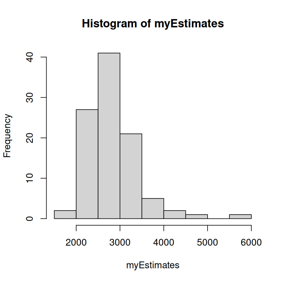
The expected value (i.e. mean) number of stickers that is required to complete an album of 427 stickers is in fact \(427 \times H_{427}\), where \(H_{427}\) is the 427\(^{th}\) Harmonic number (the mathematics of this is explained in the info box below if you are interested).

It turns out that \(H_{427} \approx 6.635\), and so the estimated mean is about 2,800 or so. This is a lot of stickers! The requisite number would be reduced in practice, because you are able swap duplicate stickers with your friends, as well as send off to Panini on a special form for a maximum of 50 stickers towards the end, but nevertheless, this simulation has explained my disappointment as a 9-year-old child!

Show: Relating sticker collecting to the harmonic numbers

In the lecture I claimed that the example of collecting things is somehow related to the harmonic series. To see this does not require sophisticated mathematics.

If there are a total of \(N\) stickers, of which you have already collected \(M\), the probability of a new sticker being one you “need” is \(p_{M} = (N-M)/N\). Assuming that successive purchases are independent, the number of stickers that must be bought to get a sticker you need when you already have \(M\) stickers in your album would follow a geometric probability distribution⁵. The expected number of stickers needed to get the \(M^{th}\) sticker is therefore \(\frac{1}{p_{M}}\).

The number of stickers that you must buy to complete the entire album is then just the expected number of stickers to get the first sticker in your album (i.e. when you have already got 0), plus the expected number required for your second sticker (i.e. when you have already got 1), …, all the way up to the expected number to get the final sticker (i.e. when you have already got \(N – 1\)).

Therefore \[\text{Average number of stickers required} = \frac{1}{p_{0}} + \frac{1}{p_{1}} + \dots +\frac{1}{p_{N-1}}.\]

However (by the definition of \(p_{M}\)) this reduces to \[\begin{aligned} \text{Average number of stickers required} &= \frac{N}{N} + \frac{N}{N-1} + \dots + \frac{N}{1} \\ &=N\left(\frac{N}{N} + \frac{N}{N-1} + \dots + \frac{1}{1}\right) \\ &=N\left(1 + \dots + \frac{1}{N-1} + \frac{1}{N}\right) \\ &=N \times H_{N}\end{aligned} \]

where we reversed the order of the sum in going from line 2 to line 3, and have used the definition of the \(N^{th}\) harmonic number (see lecture slides) on line 4.

3.9.2 Extended example two: the logistic map

[Note this task is optional, and you should do it only if you have time]

The logistic map is a simple population model in discrete-time, and relates the size of a population in generation \(n+1\) to its size in generation \(n\). It is one of the simplest models that shows “chaotic” behaviour.

One way of writing the logistic map is via the following recurrence \[x_{n+1} = rx_{n}(1-x_{n})\] where \(x_{n}\) is the population size in year \(n\), measured as a fraction of the carrying capacity, and \(r\) is the intrinsic rate of increase (a growth rate).

Task

What do you think is the purpose of the following function?

logisticValues <- function(r, N, x0) { 
  retVal <- numeric(N)
  thisX <- x0
  for(i in 1:N) { 
    thisX <- r * thisX * (1 - thisX)
    retVal[i] <- thisX 
  }
  return(retVal) 
} 

Solution

The given function returns \(N\) iterates of the logistic map starting at \(x_0\) (note, it does not store the initial value).

Copy the function logisticValues into your script file. Also include the following code that uses the function to plot a graph.

r <- 1.5        # growth rate
N <- 100        # max generation
x0 <- 0.01      # initial value
xn <- logisticValues(r, N, x0)  # next N starting at x0 
plot(0:N, c(x0, xn), type = 'o', xlab = 'n', ylab = 'x_n')  # plot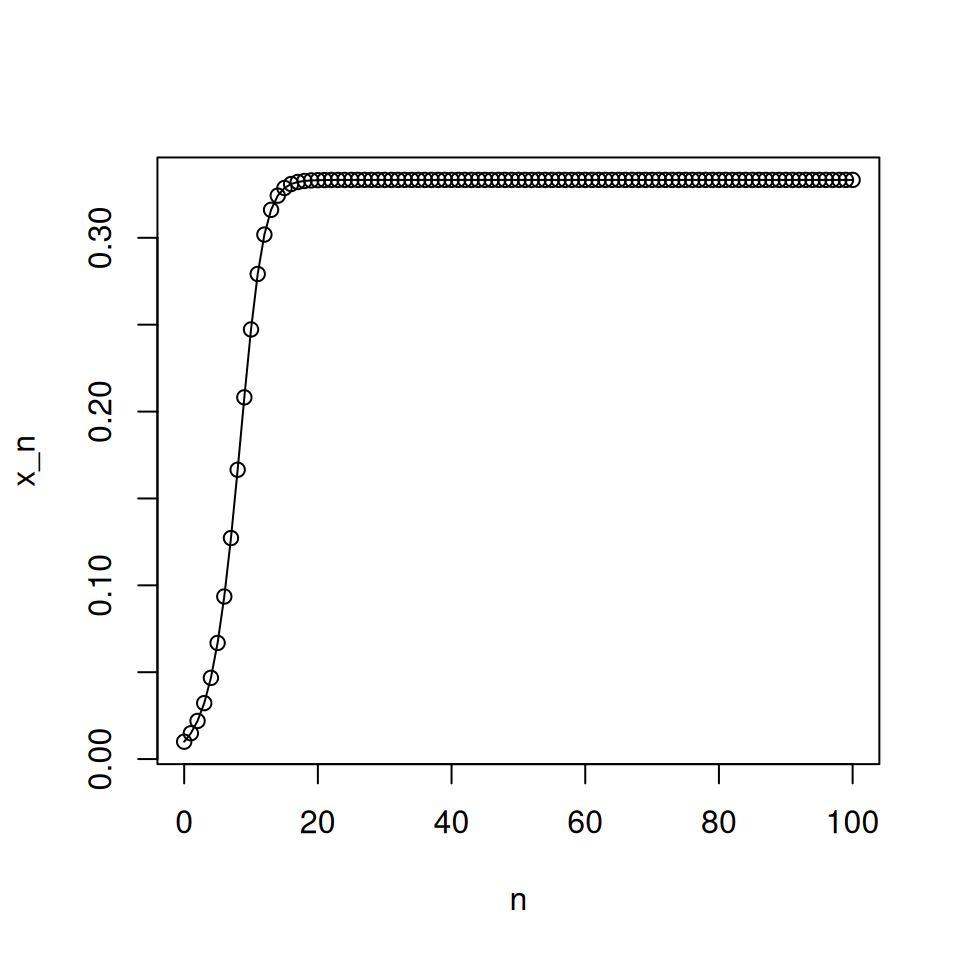

This code shows the behaviour of the logistic map with \(r = 1.5\) for 100 generations. Note the slightly clunky way of making sure the initial point is returned.

Task

Try running the code for different values of \(r\). What does the graph show you?

Good values of \(r\) to try would be \(r = 0.5\), \(r = 1.5\), \(r = 2.5\), \(r = 3.1\), \(r = 3.5\), \(r = 3.7\). You should also test the behaviour for different initial conditions: suitable values would be \(x_{0} = 0.01\) and \(x_{0} = 0.1\).

Solution

As you change the value of \(r\) in the above code the system goes from having a single equilibrium in the long term, to oscillating between a pair of values, to oscillating between four values. By \(r = 3.7\), the trajectory depends very sensitively to the initial value \(x_0\) (as is demonstrated by the below code). This is called deterministic chaos.

You should note that in the case \(r = 3.7\), the pattern of successive population sizes appears to be fairly random. It also depends on the initial value of \(x_0\). The following code confirms this (note the first five lines are almost exactly as they were before): include this code in your script to check this.

r <- 3.7            # growth rate
N <- 100            # max generation
x0 <- 0.01          # initial value
xn <- logisticValues(r, N, x0)    # next N starting at x0
plot(0:N, c(x0, xn), type = 'o', xlab = 'n', ylab = 'x_n') # plot 
x0 <- 0.01001       # different initial value
xn <- logisticValues(r, N, x0)    # next N starting there
lines(0:N, c(x0, xn), type = 'o', col = 'red') # overlay on plot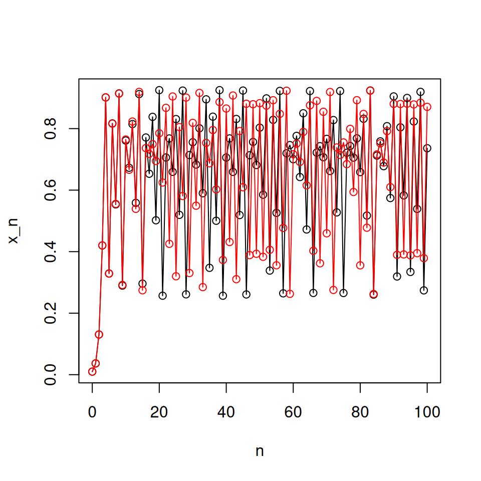

Notice that, despite starting very close together, the trajectories diverge over time. “Sensitive dependence on initial conditions” is characteristic of deterministic chaos.

Task

What do you think the following code does?

Test your understanding by typing the function in and running it by issuing an appropriate call to the function at the command prompt.

logisticValuesAfterBurnIn <- function(r, N, M, x0) { 
  retVal <- numeric(M)
  thisX <- x0
  for(i in 1:N) { 
    thisX <- r * thisX * (1 - thisX)
  }
  for(i in 1:M) { 
    thisX <- r * thisX * (1 - thisX)
    retVal[i] <- thisX 
  }
  return(retVal) 
} 

Solution

The given code performs \(N\) iterations of the logistic map starting from \(x_0\) but does not store them. It then calculates, stores and returns the following \(M\) iterations of the logistic map.

Enter the following code and run it.

rVals <- seq(2.5, 4, by = 0.005)
plot(c(2.5, 4), c(0, 1), type = 'n', xlab = 'r', ylab = 'orbit')
for(r in rVals) { 
  N <- 1000     
  M <- 100 
  xn <- logisticValuesAfterBurnIn(r, N, M, 0.01)
  points(rep(r, M), xn, pch = 19, cex = 0.01)
} 

Question

Do you understand what the plot—a so-called “bifurcation diagram”—is showing?

Answer

The key idea is that, for each value of \(r\), it calculates \(N=1000\) iterations of the map, but totally ignores them. It then plots the values of the next 100 iterations (as the \(y\)-value on a graph which has the value of \(r\) as the \(x\)-ordinate). The idea behind all this is to let the system equilibriate—if it is ever going to do so. So from the bifurcation diagram you can see from this picture that there is/are:

• a single equilibrium for \(2.5 < r < 3.0\)
• two equilibria for \(3.0 < r < 3.45\) (-ish)
• four equilibria for \(3.45\)(-ish) \(< r < 3.54\) (-ish)
• by \(r \sim 3.57\), we have chaos (as seen in plots for different starting conditions above) which here corresponds to a more or less random—although lying within certain bounds—set of 100 points plotted for each \(r\).

This is explained well on the relevant Wikipedia page

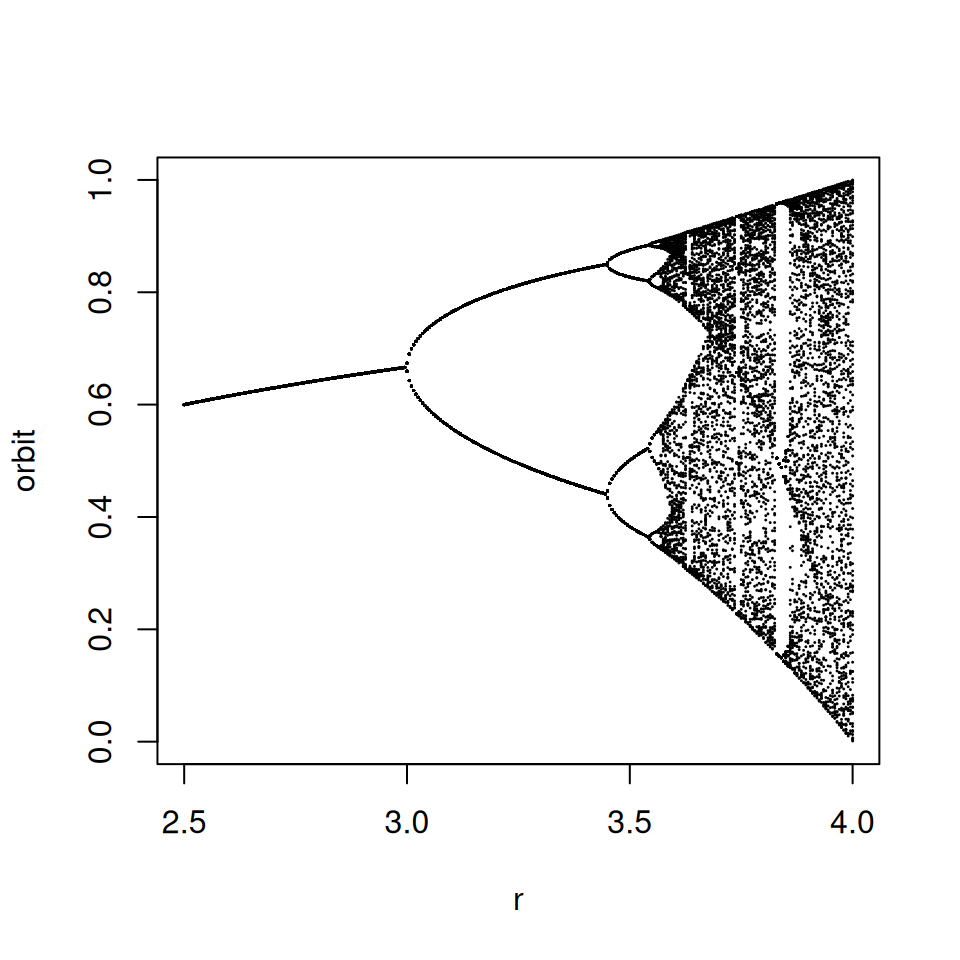
A very readable introduction to deterministic chaos in biology is given by May (1976). That article is widely available online and comes highly recommended.

---

5. You will be reminded of basic facts about probability distributions in a forthcoming lecture. Note the expected number is quite intuitive: as a simple example, consider rolling a dice until you get a six. The probability of getting a six is \(\frac{1}{6}\): hopefully it seems reasonable that you should have to roll the dice an average of 6 times to get one. That’s all that is happening here, just written in symbols.↩︎