13 Outbreak of influenza in a boarding school

Andrew Conlan (ajkc2@cam.ac.uk)

13.1 Data summary and challenge

In this practical you will calibrate a transmission model to describe the outbreak of influenza in a English boarding school.

For the purposes of this practical assume that the numbers of pupils in bed measure the numbers infectious on each date. Not a great assumption as they are to an extent self-isolating, but also not terrible given the relatively short latent and (effective) infectious period for influenza (\(\sim 1\) day).

Model the likely impact on the outbreak should 80% of the boys have been vaccinated before the start of the outbreak with a vaccine with 50% (direct) protection from infection.

Note

For a single outbreak it is reasonable to neglect the potential for loss of immunity to reinfection so modelling vaccination in this case only amounts to changing the initial conditions of the model (i.e. the number susceptible and recovered when infection is introduced.) We are told to assume an exposed period of 1 hour and an infectious period of 2 days so a standard \(SEIR\) compartmental model should be sufficient. You should use a deterministic model for your initial calibration and the explore how the dynamics differ for the corresponding stochastic model.

require(outbreaks)
require(tidyverse)
require(deSolve)

ggplot(influenza_england_1978_school,aes(x=date,y=in_bed)) + geom_point() + geom_line() + xlab('Date') + ylab('In Bed (Assumed Infectious)')

targetI <- influenza_england_1978_school$in_bed

Show: Deterministic model

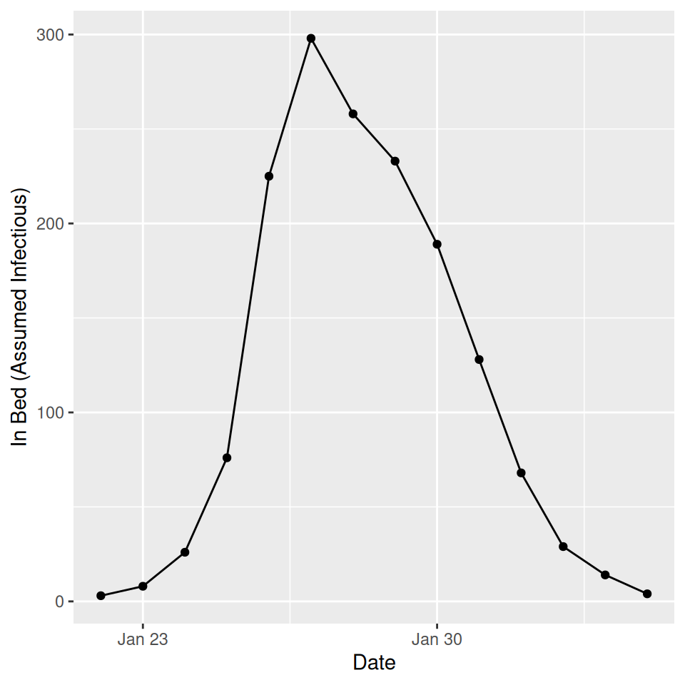
For the standard \(SEIR\) model with constant rates of progression through the exposed and infectious compartments an \(R_0\) of \(\sim 4.0\) gives a rough calibration to the observed data (black points and lines):

SEIR_gamma <- function(t,y,theta) {
  
  x_i = integer(2);
  beta = theta[1];
  TE = theta[2];
  TI = theta[3];
  x_i[1] = theta[4];
  x_i[2] = theta[5];
  
  I_tot=0;
  N_tot=0;
  
  dy_dt = numeric(2+x_i[1]+x_i[2]);
  
  for(k in (1+x_i[1]+1):(1+x_i[1]+x_i[2])){I_tot = I_tot + y[k];}
  for(k in 1:(2+x_i[1]+x_i[2])){N_tot = N_tot + y[k];}
  
  lambda = beta*I_tot/N_tot
  
  #Susceptibles      
  dy_dt[1] =  - (lambda) * y[1];
  #First stage of Exposed (but not yet infectious)
  dy_dt[2] =  lambda * y[1]  - (x_i[1]/TE) * y[2];
  
  #If shape parameter > 1 update internal exposed stages
  if(x_i[1]>1){
    for(k in 3:(1+x_i[1]))
    {dy_dt[k] = (x_i[1]/TE) * y[k-1] - (x_i[1]/TE) * y[k];}
  }
  #First infectious stage
  dy_dt[(1+x_i[1]+1)] = (x_i[1]/TE)*y[(1+x_i[1])] - (x_i[2]/TI)*y[(1+x_i[1]+1)];
  #If more than one infectious stage, run through internal stages
  if(x_i[2]>1)
  {
    for(k in (3+x_i[1]):(1+x_i[1]+x_i[2]))
    {dy_dt[k] = (x_i[2]/TI) * y[k-1] - (x_i[2]/TI) * y[k];}
  }
  
  # Final absorbing recovered stage
  dy_dt[(1+x_i[1]+x_i[2]+1)] = (x_i[2]/TI)*y[(1+x_i[1]+x_i[2])];
  
  
  return(list(dy_dt))
}

det_SEIR <-function(R0,TE,TI,shape_E,shape_I,vacc)
{
  N0 = 763.0
  
  theta = numeric(5)
  
  beta = R0/TI
  s0 = (1-vacc)*(N0-1)
  e0 = 1
  i0 = 0
  r0 = vacc*(N0-1)
  
  y0 = numeric(2+shape_E+shape_I);
  y0[1] = s0;
  y0[2] = 1
  y0[2+shape_E+shape_I] = r0
  
  theta[1] = beta;
  theta[2] = TE;
  theta[3] = TI;
  theta[4] = shape_E
  theta[5] = shape_I
  
  y<-lsoda(y0,seq(0,30,1),SEIR_gamma,theta)
  #y0 = y[dim(y)[1],2:(3+shape_E+shape_I)]
  #y<-lsoda(y0,seq(0,prevacc*364,1),SEIR_gamma,theta)
  
  # return total number infected
  
  if(shape_E==1 & shape_I==1)
  {return(y[,4])
  }else if(shape_E==1 & shape_I > 1)
  {
    return(rowSums(y[,(2+1):(2+1+shape_I)]))
  }else if(shape_E> 1 & shape_I == 1)
  {
    return(y[,(2+shape_E+1)])
  }else
  {
    return(rowSums(y[,(2+shape_E+1):(2+shape_E+shape_I)]))
  }

}

# Standard SEIR model (exponential latent, infectious periods)

expI <- det_SEIR(2.0,0.04,2.0,1,1,0.0)
det_calibrate <- tibble(time=1:14,var='R0 = 2',I=expI[1:14])

expI <- det_SEIR(4.0,0.04,2.0,1,1,0.0)
det_calibrate <- det_calibrate %>% bind_rows(tibble(time=1:14,var='R0 = 4',I=expI[1:14]))

expI <- det_SEIR(5.0,0.04,2.0,1,1,0.0)
det_calibrate <- det_calibrate %>% bind_rows(tibble(time=1:14,var='R0 = 5',I=expI[1:14]))


ggplot(det_calibrate,aes(x=time,y=I,col=var)) + geom_line() + geom_point() + 
  annotate('point',1:14,targetI[1:14]) + annotate('line',1:14,targetI[1:14])

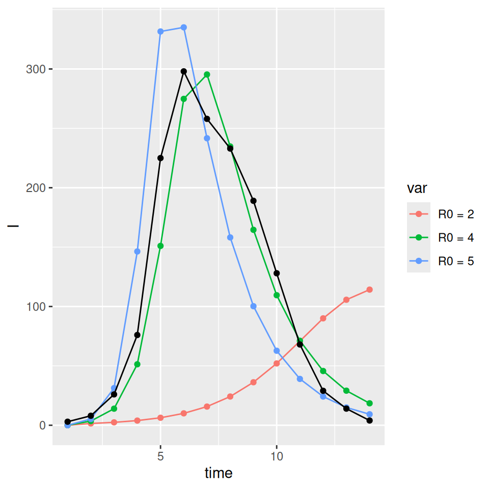
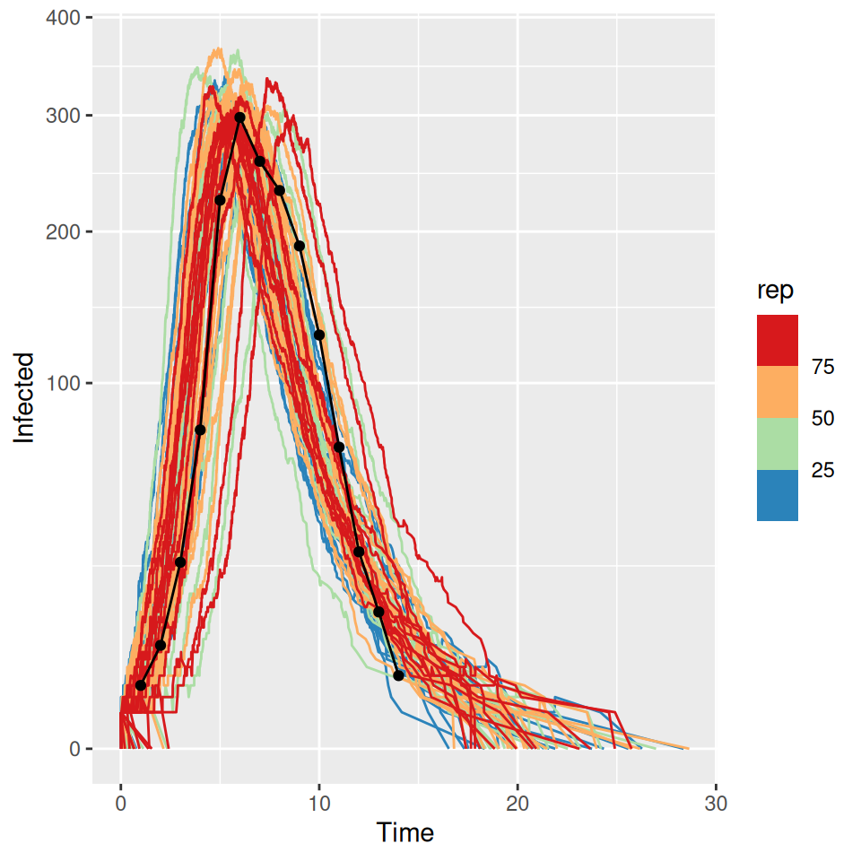
This rough calibration does not hold up if we now vary the distributional assumption for the latent and infectious periods. The supplied code has implemented the \(SEIR\) model with gamma distributed (strictly an Erlang distribution were the shape parameter is an integer) latent and infectious periods. If we vary the shape parameters for I and E we see that the peak prevalence and initial rate of exponential growth are very sensitive to changes in the distribution. Less dispersed distributions (i.e. higher shape parameters) have sharper epidemics with higher peak prevalence. The final size (and approximate value of \(R_0\)) on the other had are insensitive to these changes. Below we plot a set of three curves below for shape parameters = 10 illustrating that we now require a lower value of \(R_{0}\) to (roughly) match the data. The fit is not as good as I deliberately picked the average infectious and latent periods to give a reasonable fit with the exponential model…

# Standard SEIR model (gamma 10 latent, infectious periods)

expI <- det_SEIR(2.5,0.04,2.0,10,10,0.0)
det_calibrate <- tibble(time=1:14,var='R0 = 2.5',I=expI[1:14])

expI <- det_SEIR(2.75,0.04,2.0,10,10,0.0)
det_calibrate <- det_calibrate %>% bind_rows(tibble(time=1:14,var='R0 = 2.75',I=expI[1:14]))

expI <- det_SEIR(3.0,0.04,2.0,10,10,0.0)
det_calibrate <- det_calibrate %>% bind_rows(tibble(time=1:14,var='R0 = 3',I=expI[1:14]))


ggplot(det_calibrate,aes(x=time,y=I,col=var)) + geom_line() + geom_point() + 
  annotate('point',1:14,targetI[1:14]) + annotate('line',1:14,targetI[1:14])

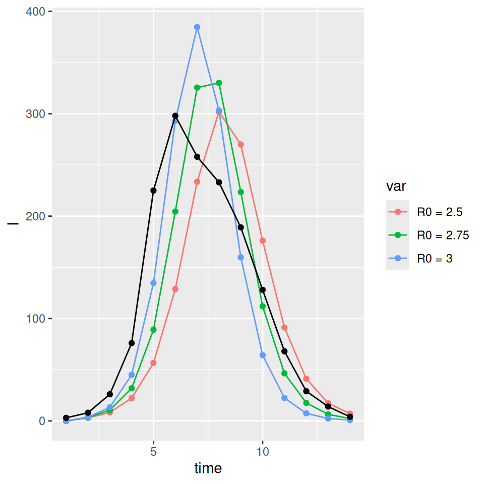
In practice the latent and infectious period distributions are not identifiable purely from a single epidemic curve. As this very simple comparison demonstrates calibrating our model based on the wrong assumption can lead to a significant under or over estimate of \(R_{0}\).

Show: Stochastic model

The rough calibration we identified using the deterministic model mostly holds up for the stochastic model with replicates scattering around the observed numbers. Although the population is small, the transmission rate is relatively high (\(R_{0}=4\)) so the deterministic model is a reasonable approximation for the average of the stochastic simulations. If the transmission rate was lower this would not necessarily be the case.

SEIR_rates <- function(state,p)
{ 
rate <- numeric(2)
# Probability of a transmission sum(state) = population size N
rate[1] <- p['beta']*state['S']*state['I']/sum(state)
# Probability of emergence from E to I
rate[2] <-p['sigma']*state['E']
# Probability of recovery from I to R
rate[3] <-p['gamma']*state['I']
return(rate) 
}

SEIR_events <- function(state,rate)
{
    total_rate <- sum(rate)
    # Draw single random variate
    x <- runif(1)
    if(x*total_rate < rate[1])
    { # Transmission
      state['S'] = state['S'] - 1
      state['E'] = state['E'] + 1
    }else if(x*total_rate < sum(rate[1:2]))
    { # Emergence
      state['E'] = state['E'] - 1
      state['I'] = state['I'] + 1
    }else{
      # Recovery
      state['I'] = state['I'] - 1
      state['R'] = state['R'] + 1
    }
    return(state) 
  }

stochastic_rep_SEIR <- function(R0,TE,TI,vacc,tmax)
{
n0 = 763.0
i0 = 1
# State Vector (One variable)
state <- c('S'=round((n0-1)*(1-vacc)),'E'=0,'I'=i0,'R'=round(vacc*(n0-i0)))
# Parameters
p = c('beta'=R0/TI,'sigma'=1/TE,'gamma'=1/TI)

# Time Variable
t <- 0.0;
# Save I and R only (I to compare to data, R to calculate final size)
# Could record all states but will be more costly in terms if memory use and run time
# so omitted here.
# Subtract off initial number vaccinated so that R counts total cumulative infections
output <- tibble(t=0,I=state['I'],R=state['R']-round(vacc*(n0-i0)))

# Calculate initial rate of events
rate_vector <- SEIR_rates(state,p)
total_rate = sum(rate_vector)
# Main Loop
repeat
{ 
  # Update time - sample time increment from from exponential distribution
  # with rate given by total rate
  t = t + rexp(1,total_rate)
  # Simulate the event using relative rates in rate_Vector
  state <-SEIR_events(state,rate_vector)
  # Output
  output <- output %>% bind_rows(tibble(t=t,I=state['I'],R=state['R']-round(vacc*(n0-i0))))
  # Calculate rate of events
  rate_vector <- SEIR_rates(state,p)
  total_rate = sum(rate_vector)
  if(t > tmax || total_rate == 0){break}
} 
return(output)
}  

out <- tibble()

for(i in 1:100) {
    out <- out %>% bind_rows(stochastic_rep_SEIR(4.0,0.04,2.0, 0.0, 30) %>% mutate(rep=i))
}

ggplot(out,aes(x=t,y=I,col=rep,group=rep)) + geom_path() + scale_y_sqrt() + 
  annotate('point',1:14,targetI[1:14]) + annotate('line',1:14,targetI[1:14]) + 
  scale_color_fermenter(palette = "Spectral") + xlab('Time') + ylab('Infected')

outvacc <- tibble()

for(i in 1:100) {
    outvacc <- outvacc %>% bind_rows(stochastic_rep_SEIR(4.0,0.04,2.0, 0.8, 30) %>% mutate(rep=i))
}

outagg <- (out %>% mutate(vacc=FALSE)) %>% bind_rows(outvacc %>% mutate(vacc=TRUE))

ggplot(outagg,
       aes(x=t,y=I,col=vacc)) + geom_path() + xlab('Time') + ylab('Infected') + scale_y_sqrt()

The main reason for considering a stochastic model for this question is then to quantify how vaccination changes the chances of seeing an outbreak at all. We can calculate this from our simulated scenarios by calculate the mean number of simulations that have more than one infection ( mean(outbreak) in table below) or compare the final size distribution for the two scenarios.

outagg %>% 
    group_by(rep,vacc) %>% 
    summarise(outbreak=max(R)>1) %>% 
    ungroup() %>% 
    group_by(vacc) %>% 
    summarise(mean(outbreak))

## # A tibble: 2 × 2
##   vacc  `mean(outbreak)`
##   <lgl>            <dbl>
## 1 FALSE             0.75
## 2 TRUE              0.36

ggplot(outagg %>% 
        group_by(rep,vacc) %>% 
        summarise(fsize=max(R)),
    aes(x=vacc,y=fsize)) + 
        stat_summary(fun.data = "mean_cl_boot")