8 Epidemic models—Practical 3

Matt Castle (mdc31@cam.ac.uk) and Andrew Conlan (ajkc2@cam.ac.uk)

8.1 Stochastic models

Aim: To explore the effects of stochasticity on simple \(SI\) and \(SIR\) models and contrast their behaviour with previous deterministic results.

Goals:

By the end of this practical participants should be able to achieve the following:

• Code up a simple stochastic \(SI\) model in R using the SimInf package.
• Code up a simple stochastic \(SIR\) model in R using the SimInf package.
• Run both single and multiple realisations and visualise the results.
• Explore extensions to both \(SI\) and \(SIR\) models:
  • Expand the \(SI\) model to include additional transitions.
  • Understand the impact of R0 values on stochastic extinction.

Background: This practical follows on from the Stochastic Epidemic Models Lecture and echoes the content presented there.

8.2 Coding a simple \(SI\) model

We will first implement a slight modification to the code that has been presented to you in the previous Stochastic Epidemic Lecture. The key difference between the code presented in the lecture and the code shown here is that we are putting the code into a function (called StocSI.dyn) rather than just running a series of commands.

• Open Rstudio.
• Open a new blank script file.
• Save it as Stoch_SI.R.

In the script window type the following commands:

library(SimInf)

create.StocSI <- function(N, I0, beta, f_time) {
    
    initial_state <- data.frame(S = N-I0 , I = I0)
    compartments <- c("S", "I")
    transitions <- c("S -> beta*S*I/(S+I) -> I")
    tspan <- seq(from = 1, to = f_time, by = 1)
    
    model <- mparse(transitions = transitions, compartments = compartments, 
        gdata = c(beta = beta), u0 = initial_state, tspan = tspan)
    
    return(model)
}

Make sure you save your file and that your working directory is the same as the folder you have saved this into (Choose from menu Session > Set Working Directory > To Source File Location).

This code creates a function that creates a single stochastic \(SI\) model. We’ll dissect/explain the code in the next section.

Open a new blank script file.

Save it as Epi_P3.R

We’ll use this script to record all of the steps in this practical (unless otherwise indicated).

In the script window type the following commands and then run (select and press run button in RStudio):

source('Stoch_SI.R')
SImodel <- create.StocSI(500, 1, 0.5, 30)
out <- run(model = SImodel)
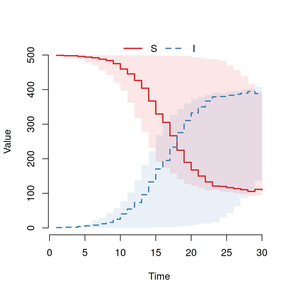
plot(out)

You should see a graph that looks similar to this:

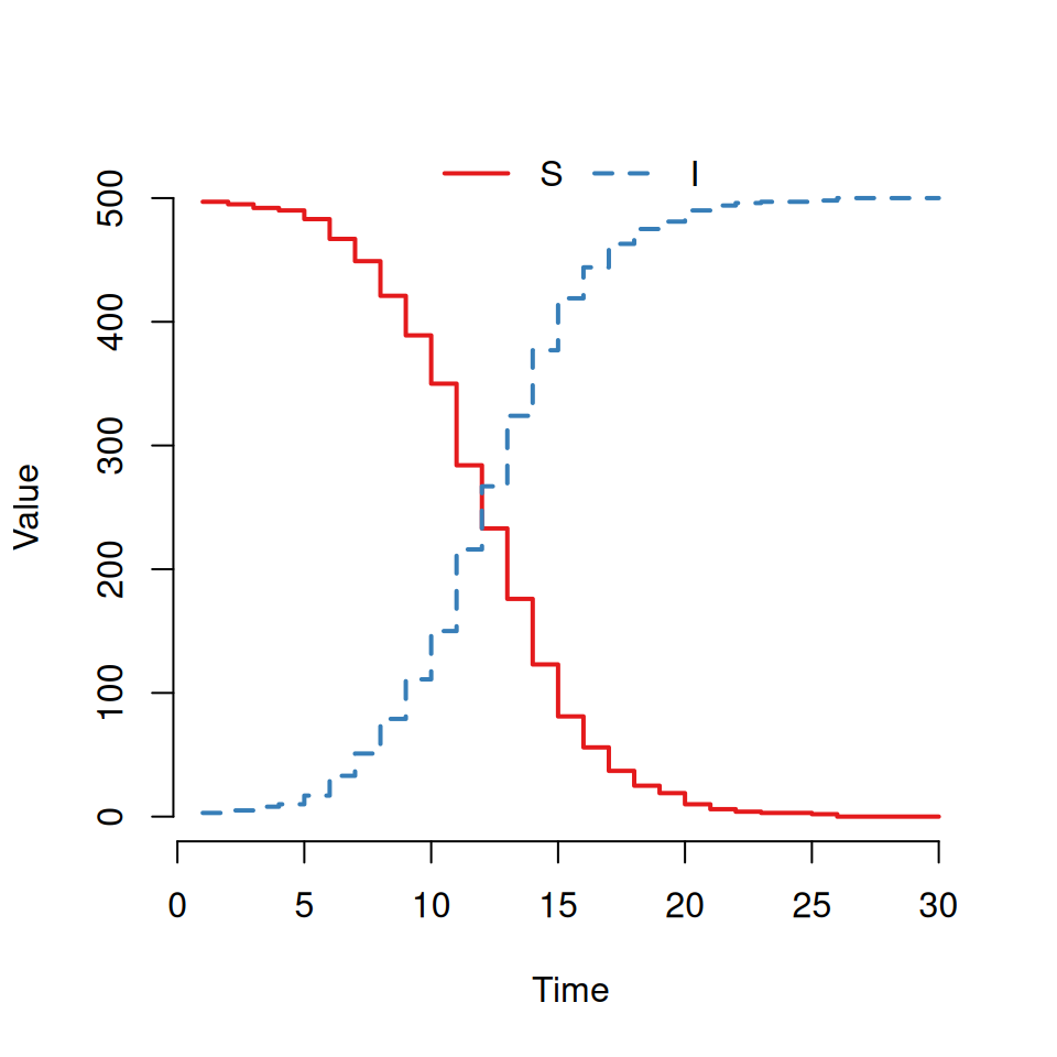
Here we can see the two trajectories for an \(SI\) epidemic. The susceptible curve (red) starts at 499 and stochastically decreases down whilst the infected curve (blue) starts at 1 and mirrors the S curve increasing stochastically.

8.3 Dissecting the stochastic \(SI\) code

The function we have just created is a wrapper that takes the basic parameters that define the \(SI\) model for a particular population and creates a R object that the SimInf package can use to simulate the model. Our function create.StocSI takes four inputs:

• Total population size: N
• Initial number of infected: I0
• Infection rate: beta
• Time to simulate for: f_time

Inside the function we combine this information to create four R objects that when passed to the SimInf function mparse. The output from the mparse function is returned as the output to our create.StocSI function.

Here we will break down what we have just written and explain what is required for the mparse function.

Note

The SimInf package includes its own function that defines \(SIR\), \(SEIR\) and \(SIS\) models (of which the \(SI\) model is a special case). The mparse function can define any generic compartmental model so it is worth learning about.

The mparse function requires that you specify the following information:

• the list of all compartments of the system
• the initial states (or compartments) of the system
• the events (or transitions) of the system
• the values of any parameters
• the time points where the value of each state is to be recorded for each simulation

An \(SI\) model is described by the following system of differential equations:

\[\begin{align} \frac{dS}{dt} &= -\beta\frac{SI}{N}\\ \frac{dI}{dt} &= \beta\frac{SI}{N} \end{align}\]

And from these equations we can derive a transition diagram from the system:

\[ S \rightarrow \beta\frac{SI}{N} \rightarrow I \]

• From this diagram we can see that there are two states for this system: susceptible and infected (S & I). We define all of the compartments of the model using a vector:

  compartments <- c("S","I")

• In order to begin the simulation, we need to specify the initial values of each compartment. We specify these using a data frame with a single row and column for each compartment specified above:

  initial_state <- data.frame(S = N-I0, I = I0)

  where N (the total population number) and I0 (the initial number of infected) have been specified by the user.

• There is one event (or transition): infection.

  transitions <- c("S -> beta*S*I/(S+I) -> I")

  where the effect is to move one susceptible into the infected compartment at a rate \(\beta \frac{SI}{N}\) where \(N=S+I\) and beta must be specified by the user. The syntax we use here should be self-explanatory (hopefully) but the idea is that we have the following syntax “A \(\rightarrow\) rate \(\rightarrow\) B” where A is the name of the starting compartment, B is the name of the ending compartment and rate explains how to calculate the rate.

• We must tell algorithm how long we want it to run for before stopping and at what points we wish to record the value of the compartments. We use the user specified variable f_time to specify a sequence of daily output values up to a maximum value of f_time.

  tspan <- seq(from = 1, to = f_time, by = 1)

  Note

  SimInf was designed to work with real epidemiological data and as such the minimum output timestep size is 1 (corresponding to 1 day).

• The mparse function takes the arguments we’ve just created, processes (‘parses’) them into a low-level computer language and compiles the resulting program into machine code. This machine code is considerably (orders of magnitude) faster than the equivalent R code. We assign the output of this function to the object SImodel (an object in R is a special data type that combines functions with data).

• Objects can be used as arguments to functions in the same way as normal data types. In this case we can use the run() function to run a stochastic simulation of the SImodel:

  out <- run(model = SImodel, threads = 1)

  The threads argument is optional here, but this argument would allow us to parallelise our code (if our setup allows it).

• The run function implements (and runs) the stochastic simulation algorithm for any stochastic model defined by the mparse function and returns a new object which contains the output of the simulation (which we’ve called out).

• The SimInf package provides a special plot function for this output

  plot(out)

This explains the code you’ve produced so far, but there are limitations. We would like to plot multiple stochastic realisations onto a single plot and investigate their aggregated properties. To do this we will need to modify our code somewhat.

8.4 Performing multiple simulations

Let’s update our create.StocSI function in the (Stoch_SI.R file) to create a model with multiple copies of the same population. This is the simplest possible meta-population model where there is no interaction between patches, and a neat hack to run multiple replicate simulations at the same time.

Edit Stoch_SI.R to update the definition of the create.StocSI as follows:

create.StocSI <- function(N, I0, beta, f_time, reps = 1) {
    
    initial_state <- data.frame(S = rep(N-I0, reps) , I = rep(I0, reps))
    compartments <- c("S", "I")
    transitions <- c("S -> beta*S*I/(S+I) -> I")
    tspan <- seq(from = 1, to = f_time, by = 1)
    
    model <- mparse(transitions = transitions, compartments = compartments, 
        gdata = c(beta = beta), u0 = initial_state, tspan = tspan)
    return(model)
}

The only two things we’ve changed here are:

1. We’ve created a new argument call reps which we’re using to specify the number of simulations that we want the code to run.

2. We’ve changed how we specify the initial_state dataframe. This is now a dataframe that has reps number of rows and 2 columns. The first column contains the starting number of susceptible individuals in each of our simulations, and the second column contains the number of initial infected individuals.

Again, remember to save your file.

Note

We have added a new argument to create.StocSI which has a default value reps = 1. By adding the argument in this way we ensure that any code we wrote earlier assuming only one replicate would still work with no modifications.

Type in the following code into Epi_P3.R and run:

#Multiple replicates
source('Stoch_SI.R')
SImodel <- create.StocSI(500, 1, 0.5, 30, 20)
out <- run(model = SImodel)
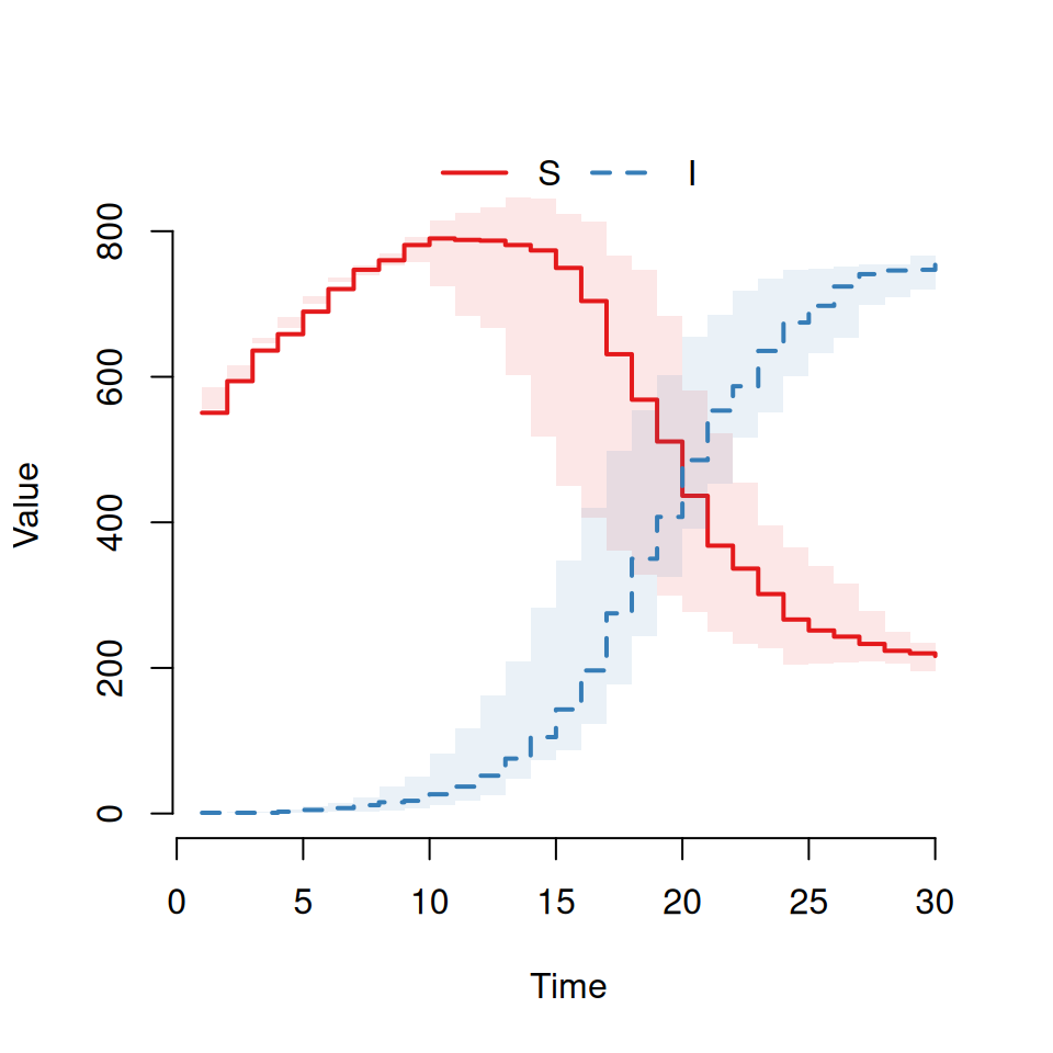
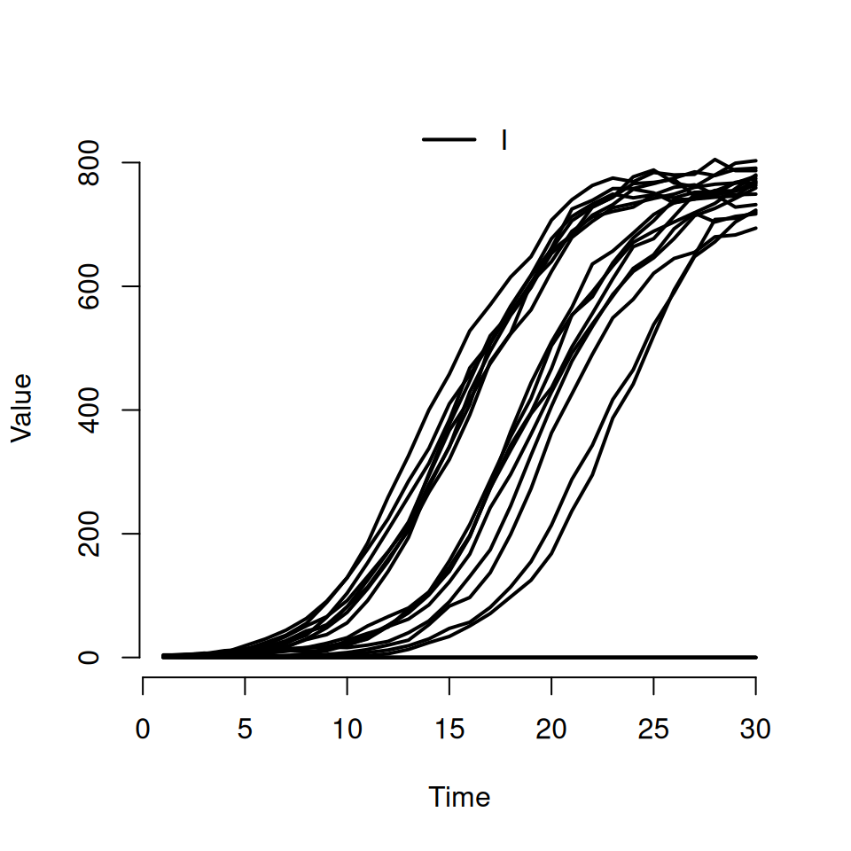
plot(out)

This should produce a plot that looks similar to the following:

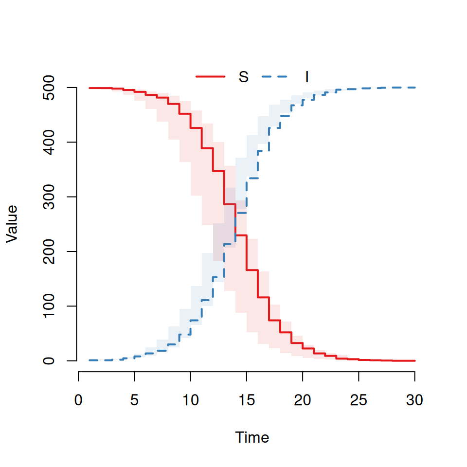
By default the plot command will always:

1. plot the curves for all states on the same graph (so we can see both \(S\) and \(I\) curves here)

2. use a step function to plot the curves (which is why it’s a bit, um, step-y)

3. show the average and interquartile range as a transparent envelope when multiple simulations have been run.

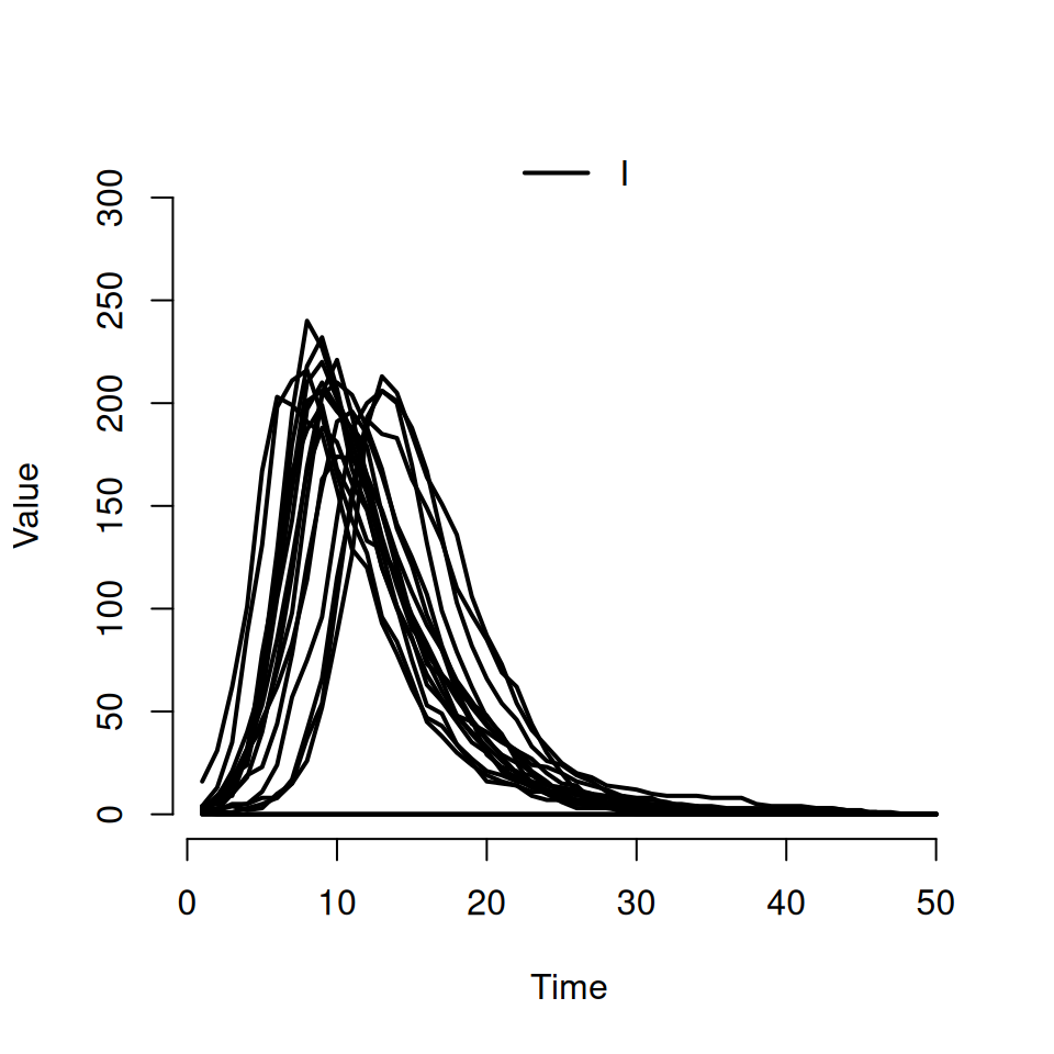
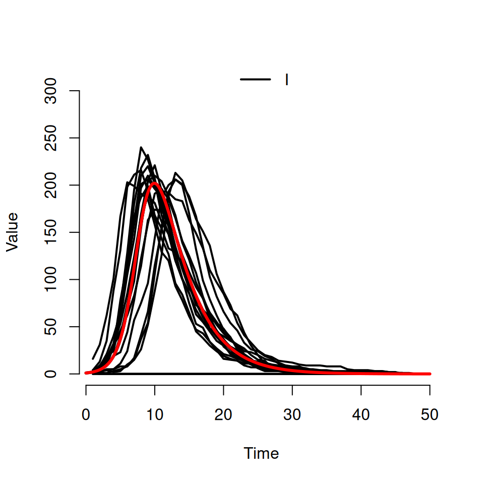
If we want to actually see individual realisations, we need to use some of the other arguments to the plot function. Try typing this in:

plot(out , 'I', range = FALSE , type = 'l')

This should produce a plot that look similar to the following:

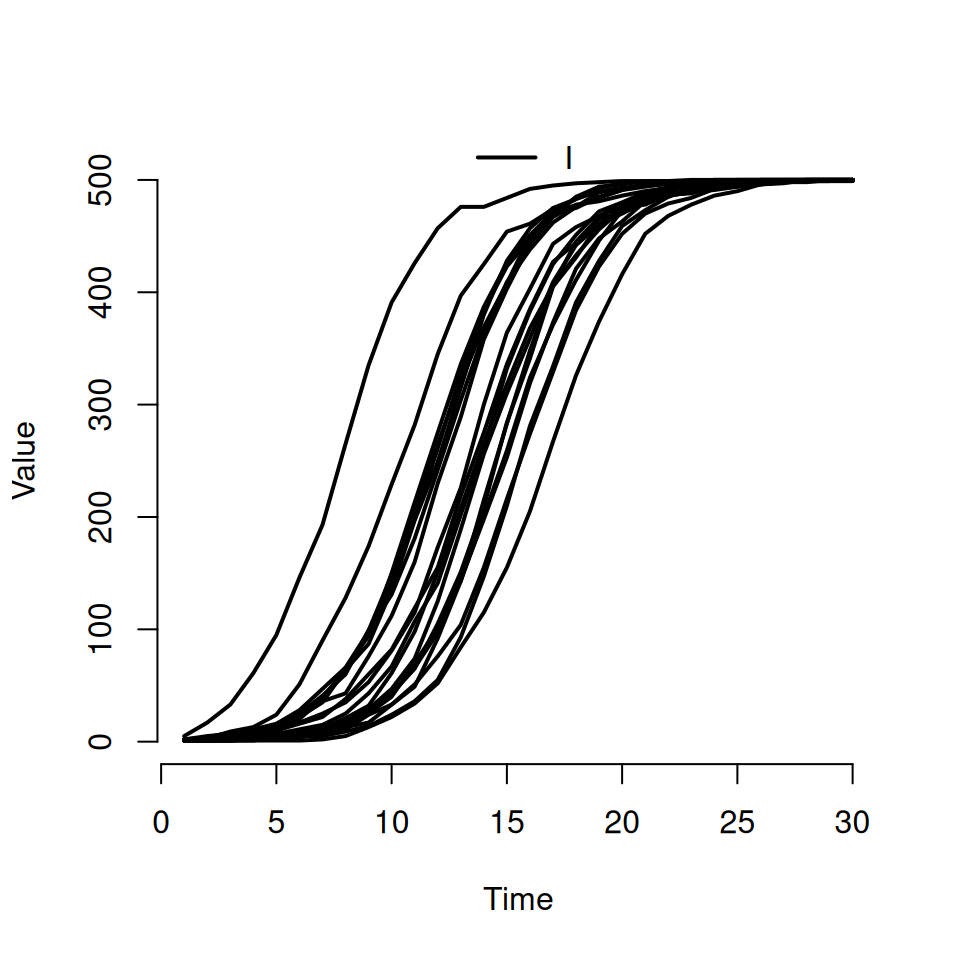
• the second argument is a character vector specifying which compartments we want to see. Here we’ve asked to only see the curves for the infected \(I\) compartment
• the named argument range is used to specify the shaded quantile on the plot. By specifying FALSE, we’ve turned it off and forced R to plot the individual trajectories instead. If we’d specified a numeric value between 0 and 1 then we would see the equivalent shaded range plotted instead (i.e. range = 0.5 corresponds to plotting the interquartile range and range = 0.95 corresponds to plotting the wider 95% quantiles)
• we can use the standard type argument from the base R plot function to specify the type of curve we want. The default is type = 's' for steps, but here we’re asking for the smoother type = 'l' lines option.

8.4.1 Adding the deterministic solution curve

Download an R script file called Det_SI.R. It contains the code for a deterministic \(SI\) model based upon the code you encountered in the first epidemic models practical. It is specifically designed to use the same parameters as have been used in the stochastic \(SI\) code written above and will add a deterministic trajectory to your plot.

Type in the following:

# adding a deterministic trajectory
source('Det_SI.R')
det.sol <- DetSI.dyn(500, 1, 0.5, 30)

det.t <- det.sol[,1]
det.I <- det.sol[,3]

lines(det.t, det.I, lwd=3 , col='red')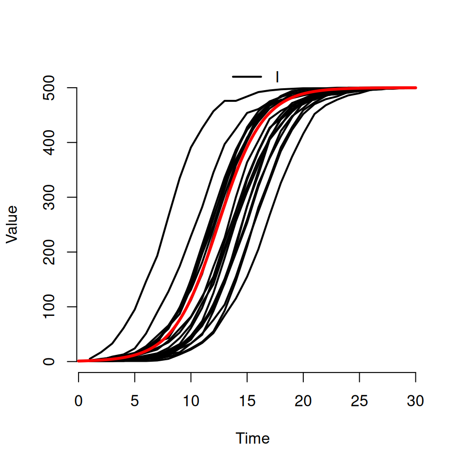

8.5 Exploring the effects of stochasticity

Task

Modify the above code to explore the effects of different initial conditions (\(I_{0} = 1, 5, 10, 50, 100\)) on the stochastic replicates. Keep the total population size constant (\(N = 500\)).

Qualitatively what effect does this have on the variability between replicates?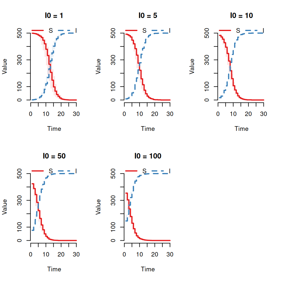

Solution

As the initial number of infectives increases the variability between replicates decreases.

ninf <- c(1, 5, 10, 50, 100)
par(mfrow = c(2, 3))
for(i in ninf) {
    SImodel <- create.StocSI(500, i, 0.5, 30, 20)
    out <- run(model = SImodel)
    plot(out, main = paste0("I0 = ", i))
}
par(mfrow = c(1, 1))

Task

Now vary the population size (\(N = 50, 500, 5000\)) with \(I_{0} = 1\).

Qualitatively what effect does this have on the variability between replicates?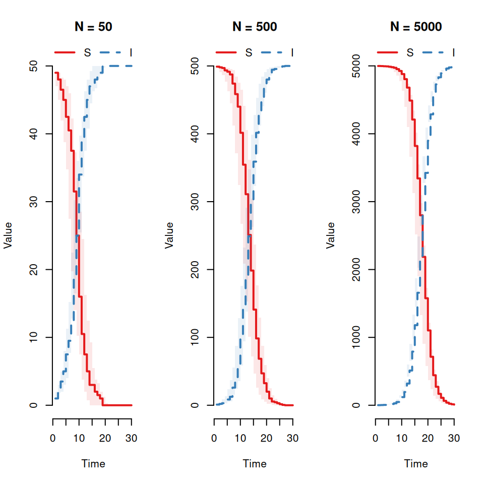

Solution

In contrast to varying the initial number of infectives, the host population size has little to no impact on the variability between replicates of the \(SI\) model. The relevant “large population” limit for the \(SI\) model is the number of infectives not the size of the host population.

npop <- c(50, 500, 5000)
par(mfrow = c(1, 3))
for(i in npop) {
    SImodel <- create.StocSI(i, 1, 0.5, 30, 20)
    out <- run(model = SImodel)
    plot(out, main = paste0("N = ", i))
}
par(mfrow = c(1, 1))

Task

Now vary the infection rate (\(\beta = 0.1, 0.5, 1\)).

Qualitatively what effect does this have on the variability between replicates?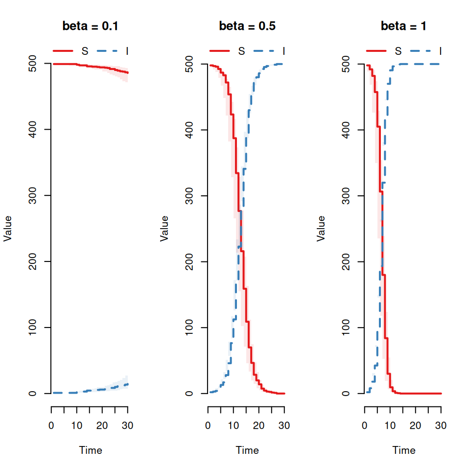

Solution

As discussed in lectures, increasing the transmission rate reduces the impact of stochasticity and the variability between replicates.

beta <- c(0.1, 0.5, 1)
par(mfrow = c(1, 3))
for(i in beta) {
    SImodel <- create.StocSI(500, 1, i, 30, 20)
    out <- run(model = SImodel)
    plot(out, main = paste0("beta = ", i))
}
par(mfrow = c(1, 1))

8.6 The delay time

Graphical exploration of model output is a good way to orientate yourself and understand the qualitative impact of changing parameters, but in practice we do need to explore various summary statistics. In this section we will compare the time it takes for a stochastic epidemic to infect half of the total population, \(t_{\frac{1}{2}}\), with the time a deterministic epidemic takes. This difference is the delay time, \(\delta t\) (see the figure below).

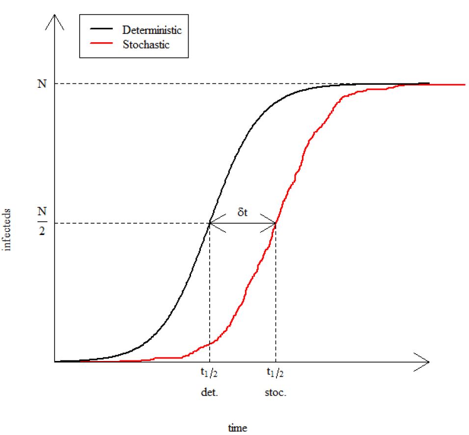
We will repeat this for many stochastic replicates and plot a distribution of the delay times.

8.6.1 The deterministic half-time

The deterministic model predicts a constant value of \(t_{\frac{1}{2}}\) given by the expression:

\[ t_{\frac{1}{2}} = -\frac{1}{\beta}\ln\left(\frac{I_{0}}{N-I_{0}}\right) \]

(This can be derived exactly from the analytic solution to the system of differential equations for the \(SI\) system. This isn’t going to be possible for more complex models.)

8.6.2 The stochastic half-time

We must now construct a function that calculates the value of \(t_{\frac{1}{2}}\) for a set of stochastic simulations and the corresponding delay times:

Open a new script file and save as Half_time.R with the following content:

# Deterministic Halftime Function
det_halftime <- function(N, I0, beta) {
    
    # calculate deterministic half life
    return((-1/beta)*log(I0/(N-I0)))
}

# Stochastic Halftime Function
stoc_halftime <- function(model) {
    
    no_runs = n_nodes(model)
    N = sum(model@u0[,1])
    
    # create storage vector for stochastic half lives
    thalf <- numeric(no_runs)
    
    # loop over number of replicates
    for (iSim in 1:no_runs) {
        # extract the infected time series for each simulation
        output <- trajectory(out, "I", iSim)
        
        # find the first time when the infected population is at least half the total population
        ind <- min(which(output$I>=(N/2)))
        thalf[iSim] <- output$time[ind]
    }
    
    return(thalf)
}

The function det_halftime takes three arguments:

• The total host population N
• The initial number of infected I0
• The infection rate beta

and returns the deterministic value of the time to half-height.

The function stoc_halftime takes a SimInf model object as its input and returns a vector with the time to half height of each model simulation (to nearest day).

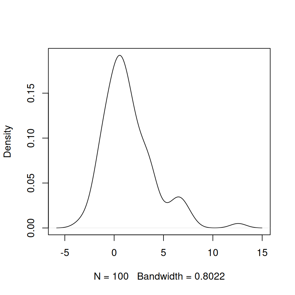
We then plot a probability density plot for these delay times using the in-built function density.

source('Half_time.R')
SImodel <- create.StocSI(500, 1, 0.5, 30, 100)
out <- run(model = SImodel)

delay_times <- stoc_halftime(out) - det_halftime(500, 1, 0.5)

plot(density(delay_times), main = '')

density produces smoothed estimates of the frequency distributions of a set of samples (essentially a smooth line through the top of a histogram). This will produce a figure similar to the one below:

Task

Can the distribution of delay-times be used to quantify the appropriateness of the deterministic approximation for a given set of parameters? In particular, in what limits will the deterministic model produce useful predictions for the time-scale of an \(SI\) epidemic? You may wish to revisit the impact of changing the host-population size N, initial number of infectives \(I_{0}\) and infection rate. Produce plots to justify your reasoning and discuss them with a demonstrator.

8.7 Coding a simple \(SIR\) model

Using the results from the earlier section on \(SI\) models as a starting point we will construct a stochastic \(SIR\) model. The deterministic \(SIR\) model equations are given by

\[ \frac{dS}{dt} = -\beta\frac{SI}{N} \] \[ \frac{dI}{dt} = \beta\frac{SI}{N}-\mu I \] \[ \frac{dR}{dt} = \mu I \]

Task

1. Using these equations construct a transition diagram for the system
2. What are the states/compartments for this system?
3. What are the transitions events and what are the rates associated with each event?
4. What is the initial state of the system (i.e. how many individuals should be in each compartment initially)?

Open a new script in RStudio.

Task

Using the functions developed in the previous sections as a template construct a create.StocSIR function that takes five arguments:

• N: the total population size
• I0: the initial number of infected individuals
• beta: the infection rate
• mu: the recovery rate
• f_time: the time the simulation will run for (daily steps)
• reps: the number of replicate simulations to run

The skeleton function below can serve as a starting point.

create.StocSIR <- function(N, I0, beta, mu, f_time, reps = 1) {
    initial_state <-
    compartments <-
    transitions <-
    tspan <-
    
    model <- mparse(transitions = transitions,
                    compartments = compartments,
                    gdata = c(beta = beta, mu = mu),
                    u0 = initial_state,
                    tspan = tspan)
    
    return(model)
}

Hint

To specify multiple transitions in the SimInf algorithm you will need a transitions vector with two elements to it like this:

transitions <- c('S -> ?? -> I', 'I -> ?? -> R')

where I have deliberately replaced the relevant transition rates with ??. You will need to replace the ?? with the correct rate equations.

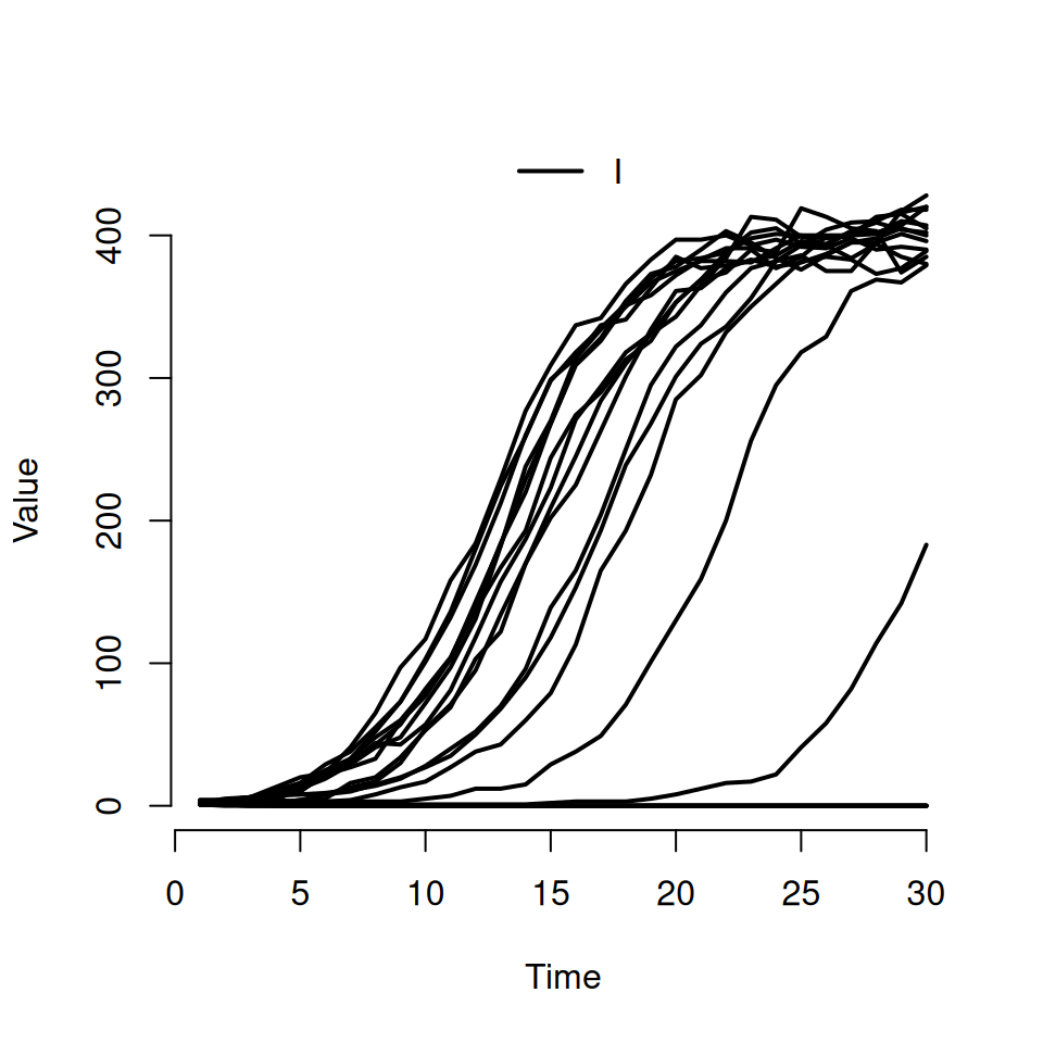
Using your function run the following code:

SIRmodel <- create.StocSIR(500, 1, 1, 0.25, 50)
out <- run(model = SIRmodel)
plot(out)

Solution

create.StocSIR <- function(N, I0, beta, mu, f_time, reps = 1) {
    initial_state <- data.frame(S = rep(N-I0, reps), I = rep(I0, reps), R = rep(0, reps))
    compartments <- c("S", "I", "R")
    transitions <- c("S -> beta*S*I/(S+I+R) -> I", "I -> mu*I -> R")
    tspan <- seq(from = 1, to = f_time, by = 1)
    
    model <- mparse(transitions = transitions,
                    compartments = compartments,
                    gdata = c(beta = beta, mu = mu),
                    u0 = initial_state,
                    tspan = tspan)
    
    return(model)
}
SIRmodel <- create.StocSIR(500, 1, 1, 0.25, 50)
out <- run(model = SIRmodel)
plot(out)

This should produce a graph that looks like this:

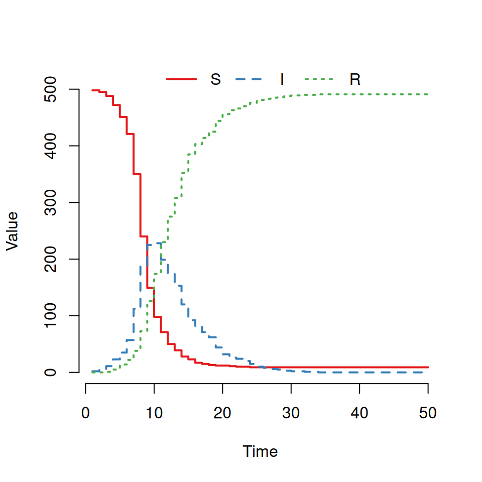
However, some of you will see a very different graph. (If you do get something like this plot then try re-running the model and plotting it several times until you see something different.)

Question

Why might this be the case?

Answer

For some replicates the initial infected individual will recover before transmitting, the disease will go extinct and there will be no epidemic.

Task

Use this function to plot 20 replicates of the infection curves (use the code in the previous \(SI\) section as a guide).

Solution

SIRmodel <- create.StocSIR(500, 1, 1, 0.25, 50, 20)
out <- run(model = SIRmodel)
plot(out , 'I', range=FALSE , type = 'l', ylim = c(0, 300))

Task

Load the R script called Det_SIR.R and adapting your code from the previous section make a plot that overlays the deterministic solution with the output of the stochastic model.

Solution

source('Materials/Epidemic_models/Functions/Det_SIR.R')
det.sol <- DetSIR.dyn(500, 1, 1, 0.25, 50)
det.t <- det.sol[,1]
det.I <- det.sol[,3]
lines(det.t, det.I, lwd = 3, col = 'red')

8.8 \(SIS\) Extension: Adding Recovery from Infection

Consider a system where individuals recover from infection with a fixed rate \(\alpha\) and return to the susceptible class. This \(SIS\) system is described by the following system of equations:

\[ \begin{aligned} \frac{dS}{dt} &= \alpha I - \beta\frac{SI}{N} \\ \frac{dI}{dt} &= \beta\frac{SI}{N} - \alpha I \end{aligned} \]

Task

1. Draw the transition diagram for this system.

2. For each transition write down the rate at which it occurs.

3. What are the parameters required for this model?

4. Write a new function create.StocSIS based upon the create.StocSI function and add to the Stoch_SI.R file and repeat the above analysis. Use these initial values for the parameters:

• \(\alpha = 0.1\)
• \(\beta = 0.5\)

Solution

create.StocSIS <- function(N, I0, alpha, beta, f_time, reps = 1) {
    initial_state <- data.frame(S = rep(N-I0, reps), I = rep(I0, reps))
    compartments <- c("S", "I")
    transitions <- c("S -> beta*S*I/(S+I) -> I", "I -> alpha*I -> S")
    tspan <- seq(from = 1, to = f_time, by = 1)

    model <- mparse(transitions = transitions,
                    compartments = compartments,
                    gdata = c(alpha = alpha, beta = beta),
                    u0 = initial_state,
                    tspan = tspan)

    return(model)
}
SISmodel <- create.StocSIS(500, 1, 0.1, 0.5, 30, 20)
out <- run(model = SISmodel)
plot(out)

plot(out , 'I', range = FALSE , type = 'l')

8.9 \(SIS\) Extension: Adding host demography

Consider an \(SI\) model with host demography. The system has constant birth rate \(\Lambda\) into the susceptible class and fixed per capita mortality rate \(\mu\) from both the susceptible and infectious classes and is governed by the following equations:

\[ \frac{dS}{dt} = \Lambda - \beta\frac{SI}{N} - \mu S \] \[ \frac{dI}{dt} = \beta\frac{SI}{N}-\mu I \]

Task

Repeat the previous steps for this model and create a create.StocSI_demo function in Stoch_SI.R and then explore its dynamics.

Hint

To specify a birth (or death) event then we use the @ symbol to represent the “empty” compartment from which births appear (or to which deaths end up). So a birth event into the susceptible compartment would have the following transition string:

@ -> ?? -> S

Use these initial values for the parameters:

• \(\mu = 0.1\)
• \(\beta = 0.5\)
• \(\lambda = 100\)

Solution

create.StocSI_demo <- function(N, I0, mu, beta, lambda, f_time, reps = 1) {
    initial_state <- data.frame(S = rep(N-I0, reps), I = rep(I0, reps))
    compartments <- c("S", "I")
    transitions <- c(
        "@ -> lambda -> S",
        "S -> beta*S*I/(S+I) -> I",
        "S -> mu*S -> @",
        "I -> mu*I -> @"
    )
    tspan <- seq(from = 1, to = f_time, by = 1)

    model <- mparse(transitions = transitions,
                    compartments = compartments,
                    gdata = c(mu = mu, beta = beta, lambda = lambda),
                    u0 = initial_state,
                    tspan = tspan)

    return(model)
}
SI_demo_model <- create.StocSI_demo(500, 1, 0.1, 0.5, 100, 30, 20)
out <- run(model = SI_demo_model)
plot(out)

plot(out, 'I', range = FALSE , type = 'l')

8.10 \(SIR\) Extension: The final epidemic size

In order to further explore the effects of stochasticity in the \(SIR\) model we are going to explore the how the final size of an epidemic varies between realisations.

• What is the final size of an epidemic?
• What does it mean?
• Which state variable do we need to consider in order to calculate the final epidemic size?

For stochastic simulations the final epidemic size will vary between realisations of the epidemic which will mean that we need to think about a distribution of final epidemic sizes.

Task

Write code to calculate the final epidemic size from a SimInf output object. Use \(\beta = 1\) and \(\mu = 0.25\) as before, running the outbreak for 50 days.

Hint

• What value should the final time for the simulations be set to (roughly)?
• As we’ve seen before, the function trajectory can be used to extract the actual values of the different compartments at each time point.
• Look at the code we used in the previous practical for calculating the halftime values for a single simulation and modify that logic accordingly.

Solution

Here we will extract the number of removals at time \(t = 50\) as an approximation of the final epidemic size.

## check for a single simulation
SIRmodel <- create.StocSIR(500, 1, 1, 0.25, 50)
out <- run(model = SIRmodel)

## extract states
u <- trajectory(out)

## find approximate final epidemic size
finalsize <- u$R[u$time == 50]
finalsize

## [1] 491

Task

Run 100 realisations, extract the final epidemic size from each one and then produce a histogram of the final sizes. It should look something similar to the figure below:

Hint

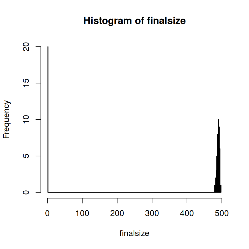
• You’ll probably want to use a loop to extract the final size for each simulation
• Set the histogram to use 500 bins

Why does the histogram have a bimodal distribution?

Solution

## run 100 replicates
SIRmodel <- create.StocSIR(500, 1, 1, 0.25, 50, 100)
out <- run(model = SIRmodel)

## extract states
u <- trajectory(out)

## find approximate final epidemic size for each replicate
finalsize <- rep(NA, 100)
for(i in 1:100) {
    finalsize[i] <- u$R[u$node == i & u$time == 50]
}
hist(finalsize, breaks = 500)

This has a bimodal distribution because as before, with a small number of initial infectious individuals there is a non-zero probability that these early infections will recover before they infect anyone else. If an epidemic does take off then the final sizes tend to cluster around the deterministic final size (\(\approx N = 500\) here).

Recall that the final epidemic size for the deterministic \(SIR\) model showed strong dependency on the value of the basic reproductive number, \(R_{0}\).

Task

• Write down an expression for \(R_{0}\) for this system as a function of the parameters \(\beta\) and \(\mu\).
• Does this help explain the bimodal result?

Solution

\[ R_0 = \frac{\beta}{\gamma} = \frac{1}{0.25} = 4. \] From the lecture notes we have that the probability of early extinction is \(P(E) \approx \frac{1}{R_0} = 0.25\). We can produce an approximation of the early extinction probabilities by counting the proportion of realisations that die out early. Based on the final size graph above, given the two very distinct modes, if we define early extinction as being any realisation with a final size \(<250\) say, then we can generate an estimate for \(P(E)\) as:

PE <- sum(finalsize < 250) / length(finalsize)
PE

## [1] 0.2

We can see that this closely aligns to our theoretical approximation.

For this section, we shall vary the value of \(R_{0}\) by varying the transmission rate, \(\beta\), whilst keeping the recovery rate, \(\mu\), at a fixed value.

Task

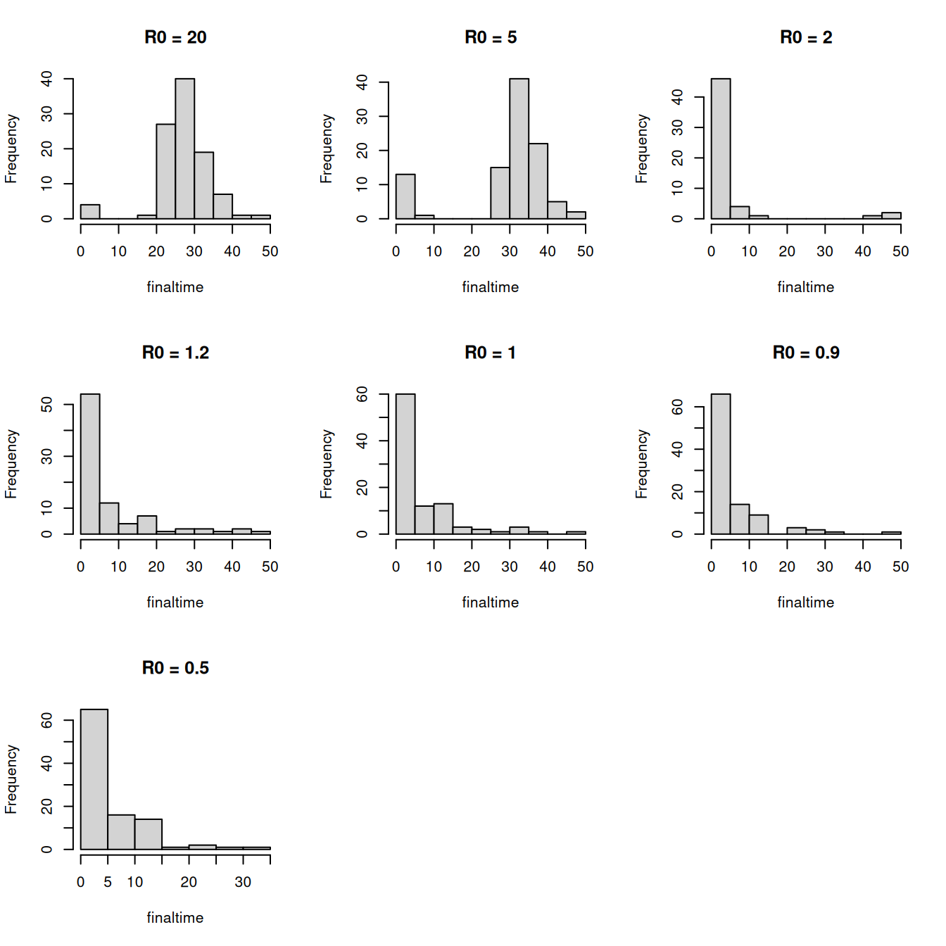
Explore how the final size distribution varies with \(R_0\) by producing histograms of the final size distribution as per the above figure for values of \(R_0 = 20.0, 5.0, 2.0, 1.2, 1.0, 0.9, 0.5\).

Can you always identify the two modes of the distribution?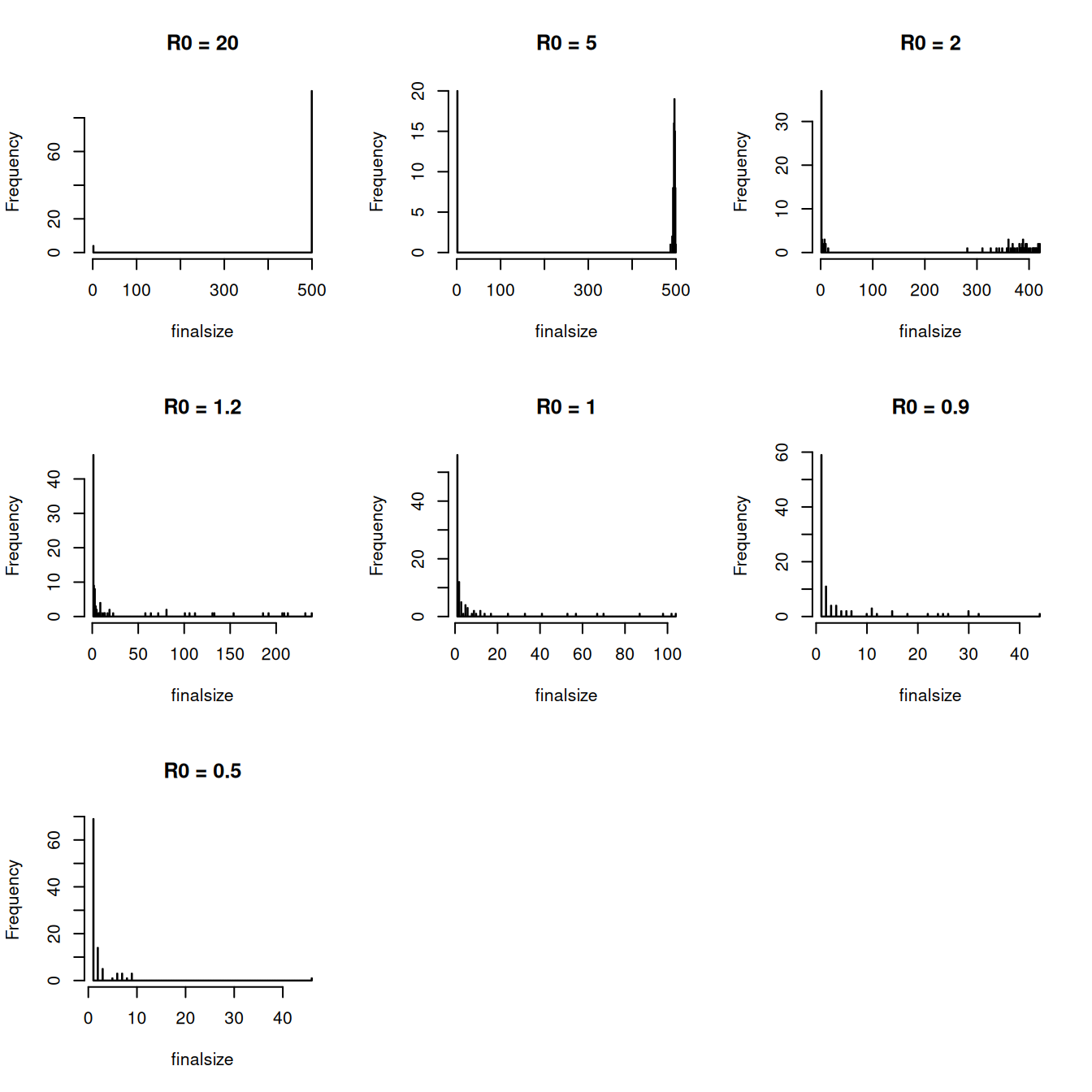

Solution

## set vector of R0 values
R0 <- c(20, 5, 2, 1.2, 1.0, 0.9, 0.5)

## set mu
mu <- 0.25

## set plot layout
par(mfrow = c(3, 3))

## loop over R0 values
for(i in 1:length(R0)) {
    
    ## calculate beta for fixed mu and R0
    beta <- R0[i] * mu
    
    ## set up and run model
    SIRmodel <- create.StocSIR(500, 1, beta, mu, 50, 100)
    out <- run(model = SIRmodel)
    
    ## extract states
    u <- trajectory(out)
    
    ## find final epidemic size for each replicate
    finalsize <- rep(NA, 100)
    for(j in 1:100) {
        finalsize[j] <- u$R[u$node == j & u$time == 50]
    }
    hist(finalsize, breaks = 500, main = paste0("R0 = ", R0[i]))
}
par(mfrow = c(1, 1))

For intermediate values of \(R_0\) the two modes will merge together.

8.11 \(SIR\) Extension: Stochastic extinction

One of the primary differences between the deterministic and stochastic formulations of the \(SIR\) model is that in the stochastic formulation the epidemic becomes extinct within a finite time, the so-called extinction time. The extinction time varies between realisations and in this section we are going to explore this distribution.

Question

Which state variable do we need to consider in order to calculate the time to epidemic extinction and what is the value of this state variable at extinction?

Answer

We should monitor the first time at which the number of infectious individuals, \(I\), equals 0.

As with the final epidemic size, the extinction time will vary over realisations of the epidemic which will result in a distribution of extinction times, which we are now going to explore.

Task

Adapt your previous code to calculate the extinction time for each realisation.

• Run 100 realisations in order to produce a histogram of the time to extinction, as per the figure below:

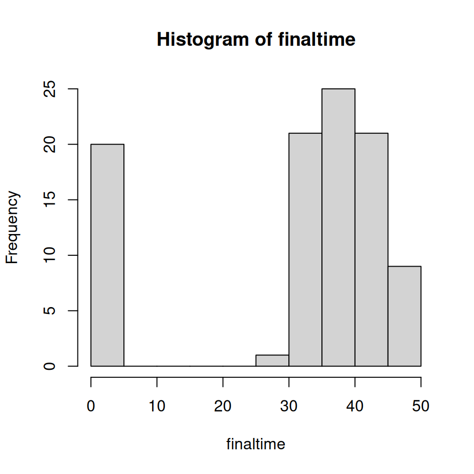
• Explore the distribution of extinction times for several values of \(R_{0} = 20.0, 5.0, 2.0, 1.2, 1.0, 0.9, 0.5\).

• What do you notice about the distribution as \(R_{0}\) gets close to 1?

Solution

To generate the first figure, consider:

set.seed(126)
## run 100 replicates
SIRmodel <- create.StocSIR(500, 1, 1, 0.25, 50, 100)
out <- run(model = SIRmodel)

## extract states
u <- trajectory(out)

## find extinction time for each replicate
finaltime <- rep(NA, 100)
for(i in 1:100) {
    ## note that this will return an NA if the epidemic hasn't ended
    finaltime[i] <- u$time[u$node == i & u$I == 0][1]
}
hist(finaltime)

To then explore how this distribution changes for different values of \(R_0\), consider:

## set vector of R0 values
R0 <- c(20, 5, 2, 1.2, 1.0, 0.9, 0.5)

## set mu
mu <- 0.25

## set plot layout
par(mfrow = c(3, 3))

## loop over R0 values
for(i in 1:length(R0)) {
    
    ## calculate beta for fixed mu and R0
    beta <- R0[i] * mu
    
    ## set up and run model
    SIRmodel <- create.StocSIR(500, 1, beta, mu, 50, 100)
    out <- run(model = SIRmodel)
    
    ## extract states
    u <- trajectory(out)
    
    ## find extinction time for each replicate
    finaltime <- rep(NA, 100)
    for(j in 1:100) {
        ## note that this will return an NA if the epidemic hasn't ended
        finaltime[j] <- u$time[u$node == j & u$I == 0][1]
    }
    hist(finaltime, main = paste0("R0 = ", R0[i]))
}
par(mfrow = c(1, 1))

As \(R_0\) gets closer to one, the extinction time distribution loses the upper mode and moves far closer to zero.