9 Estimating \(R_0\) using catalytic models

T. J. McKinley (t.mckinley@exeter.ac.uk) and Andrew Conlan (ajkc2@cam.ac.uk)

The aim of this practical is to estimate the age-stratified force-of-infection and basic reproductive ratio from age-stratified serological data for an endemic disease.

Objectives:

1. Estimate the age-stratified force-of-infection of rubella from serological data.
2. Calculate the next generation matrix and \(R_0\) for rubella.

We approach these two objectives using two alternative methods:

• In Section 9.1 we take the traditional two stage approach of estimating the force-of-infection first and then calculating the next generation matrix from an assumed Who-Aquires-Infection-from-Whom (WAIFW) matrix.
  
• In Section 9.2, we take the more elegant approach of estimating the next generation matrix directly using social contact (POLYMOD) data.

9.1 Estimating the force-of-infection and \(R_0\) of rubella

In this practical we will estimate the force-of-infection of rubella using serological survey data from the UK provided in the book “Modelling Infectious Disease Parameters Based on Serological and Social Contact Data” by Hens et al. (2012)

You will need a copy of the data (Rubella-UK.csv), which you can download via the link. We will begin by loading and checking the contents of the rubella data table:

rubella <- read.csv("Rubella-UK.csv", header = TRUE) 
head(rubella)

##   Age Pos Neg
## 1   1  31 175
## 2   2  30 116
## 3   3  34 134
## 4   4  57 132
## 5   5  95 124
## 6   6 104  91

rubella should be a table with 44 rows and 3 columns. rubella$Age is the endpoint of the age group (annual) from which rubella$Pos + rubella$Neg samples were taken, of which rubella$Pos were positive for rubella antibodies and rubella$Neg were negative.

Task

Estimate the probability of being susceptible (\(p_s\)) within each age category and add this as an extra column to the rubella data frame.

Solution

rubella$p_s <- 1 - rubella$Pos / (rubella$Neg + rubella$Pos)

The force-of-infection (\(\lambda\)) is defined as the rate that susceptible individuals acquire infection per unit time. Cross-sectional surveys provide no explicit information on how the risk-of-infection varies with time (which will depend on the epidemic dynamics), but can be used to quantify how the risk of infection depends on covariates such as age. If we assume that the individuals within an age-group experience a constant average force-of-infection then the rate of change of the proportion susceptible with age will be: \[\begin{equation} \frac{dp}{da} = -\lambda p_0 \end{equation}\] with solution: \[\begin{equation} p(a) = p_0 e^{-\lambda a} \end{equation}\] where \(p_0\) is the proportion susceptible at the beginning of the age group.

The proportion susceptible at the end of an age group, \(p_1\), will then be given by: \[\begin{equation} p_1 = p_0e^{-\lambda \Delta a} \tag{9.1} \end{equation}\] where \(\Delta a\) is the width of the age group.

Task

Take logs of both sides of (9.1) and solve for \(\lambda\) to get a first estimator for the force of the infection in a discrete age group as a function of the proportion susceptible at the beginning and end of the age group.

Show: Hint

Remember your log rules, e.g. \(\log(xy) = \log(x) + \log(y)\), \(\log\left(\frac{1}{x}\right) = -\log(x)\) and \(\log\left(e^x\right) = x\).

Solution

\[\begin{align*} &\phantom{\Rightarrow} \log\left(p_1\right) = \log\left(p_0e^{-\lambda \Delta a}\right)\\ &\Rightarrow \log\left(p_1\right) = \log\left(p_0\right) - \lambda \Delta a\\ &\Rightarrow \lambda \Delta a = \log\left(p_0\right) - \log\left(p_1\right)\\ &\Rightarrow \lambda = \frac{1}{\Delta a}\left[\log\left(p_0\right) - \log\left(p_1\right)\right], \end{align*}\] which can also be written as: \[ \lambda = \frac{1}{\Delta a}\log\left(\frac{p_0}{p_1}\right). \]

Task

Use the equation derived above to estimate the force-of-infection \(\lambda_i\) within each annual age cohort (\(i = 1, \dots, N_A\)) and add as another column to the rubella data frame (e.g. rubella$lambda).

Show: Hints

• Assume that all individuals are susceptible at birth (\(p_0 = 1\) for first age cohort).
  
• Think carefully about what the estimated force-of-infection for the final age cohort should be.
• You may wish to write a loop, or consider using vectors (e.g. 1:(nrow(rubella) - 1)) to access the different elements of rubella$p_s.

Solution

If \(\Delta a = 1\) for all age-cohorts, then the equation for \(\lambda_i\) can be estimated within each age-cohort as: \[ \lambda_i = \log\left(p_{i - 1}\right) - \log\left(p_i\right) \] for \(i = 1, \dots, N_A\) where \(p_0 = 1\). This can be implemented in R using e.g.

rubella$lambda <- log(c(1, rubella$p_s[1:(nrow(rubella) - 1)])) - 
    log(rubella$p_s)

To check your calculations and visualise the data generate the following plots:

## size is a vector to scale the size of points according to the 
## sample size within that age group 
size <- (rubella$Pos + rubella$Neg) / max(rubella$Pos + rubella$Neg) 

## now produce plots
plot(rubella$Age, rubella$p_s, pch = 19, cex = size^0.75)
plot(rubella$Age, rubella$lambda, pch = 19, cex = size^0.75)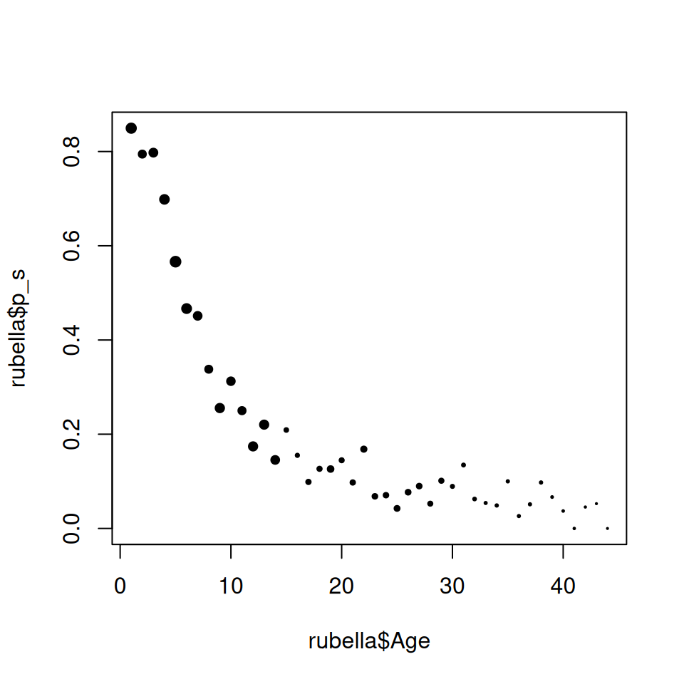

Figure 9.1: Proportion susceptible with respect to age

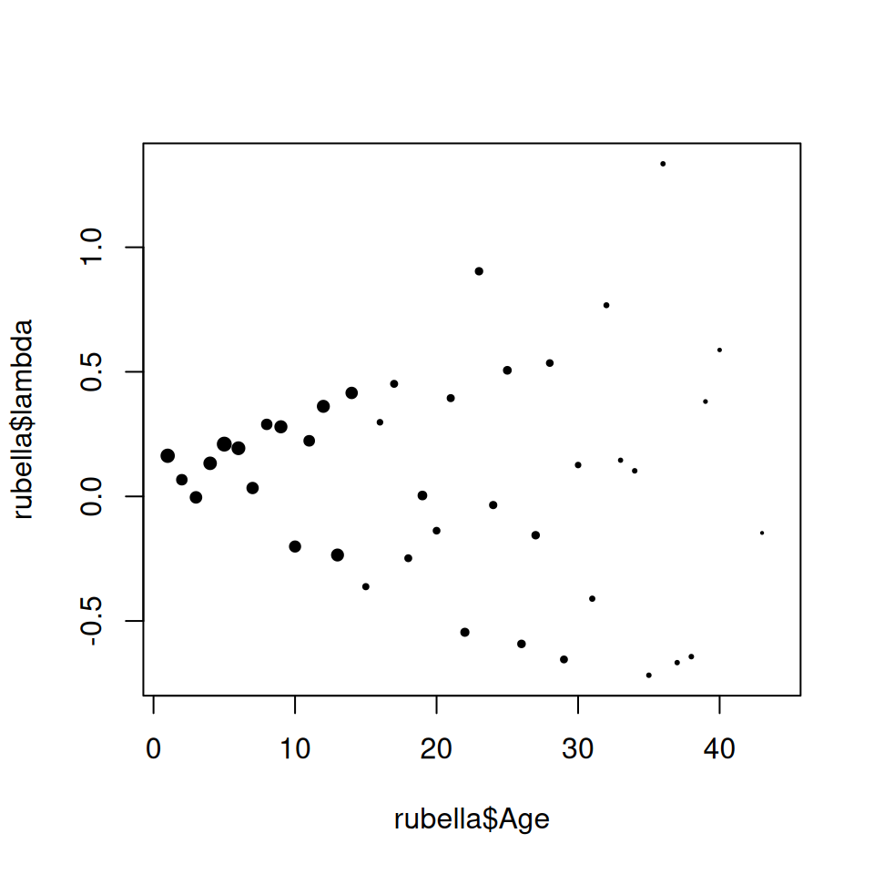
Figure 9.2: First estimate of force-of-infection of rubella

Question

Are these “first” estimates of the force-of-infection biologically plausible (Figs 9.1 and 9.2)? If not, how has this transpired and how can we improve the estimates?

Answer

Here some of the estimates of \(\lambda\) are negative, which doesn’t make sense biologically. Remember, we are crudely estimating \(\lambda\) multiple times using only information in each cohort, whilst putting no constraints on the range of values that the \(\lambda\) terms can take. We are also ignoring the fact that the susceptible proportions in each age-class are themselves estimates, and are thus measured with uncertainty. This is not a robust approach for statistical inference!

Dynamic age-structured epidemic models typically assume that the force-of-infection is constant within coarse age-groups, but can differ between age-groups. For such a coarse-grained models (with age groups of width \(a\), indexed by \(i\) as before) we can calculate the piecewise probability of remaining susceptible as introduced in lectures: \[\begin{equation} P_s(a) = \left\{\begin{array}{ll} e^{-\lambda_1 a} & \mbox{for}~a_0 < a < a_1\\ P_s\left(a_i\right) e^{-\lambda_{i + 1} \left(a - a_i\right)} & \mbox{for}~a_i < a < a_{i + 1}, \end{array}\right. \tag{9.2} \end{equation}\] where \(\lambda_i\) is the age-specific force-of-infection in group \(i\).

The function piecewise_s(a, foi) provided below returns this age-stratified probability of being susceptible at the end of each discrete age groups, specified by the vector of ages a for a given vector of force-of-infections (lambda).

## Calculate proportion of population that remains susceptible
## by age a for population with force of infection (foi)
##
## Arguments:
## a: vector of ages to calculate susceptible proportion
## lambda: vector of length equal to the maximum assumed age in the population
## with a specified force of infection for each annual cohort.  
piecewise_s <- function(a, lambda) {
    
    ## extract information on age-classes 
    max_age <- length(lambda)
    breaks <- 0:max_age
    widths <- rep(1, max_age)
    
    ## set up output vector
    s <- numeric(length(a))
    
    ## loop over age-classes
    for(i in 1:length(a)) {
        if(a[i] == 0) {
            s[i] <- 1
        } else {
            ## which age class does current value of a lie within
            age_class <- max(which(a[i] > breaks))
            sg <- 1
            if(age_class > 1) {
                ## iterate over previous age groups calculate susceptibles
                ## at beginning of age group
                for(j in 1:(age_class - 1)) {
                    sg <- sg * exp(-lambda[j] * widths[j])
                }
            }
            ## calculate susceptible proportion at age a within final
            ## age group
            s[i] <- sg * exp(-lambda[age_class] * (a[i] - breaks[age_class]))
        }
    }
    ## return vector of probabilities
    return(s)
}

The function FOI_loglik(x, foi_key, sero_data) defined below uses piecewise_s() to calculate the (binomial) likelihood of observing a given number of positive/negative samples for each age-group given in the table sero_data, for a piecewise continuous force-of-infection defined by vectors x and foi_key.

As individuals can only take two possible values, positive or negative, the likelihood of a given force-of-infection (FOI) can be written in terms of a binomial trial depending on the number of positive samples in each group (\(X_a\)), number of samples (\(N_a\)) and the predicted probability of infection within that age group (\(p_a(K)\)). Hence the log-likelihood can be written as: \[\begin{equation} l(K) = \sum_{a} \log{N_a \choose X_a} + X_a\log\left[p_a(K)\right] + \left({N_a - X_a}\right)\log\left(1 - p_a(K)\right). \end{equation}\]

We can code this in R using the following function:

## Calculate (Binomial) likelihood of observing given number of 
## positive/negative samples (provided in table sero_data) for each 
## age group and specified by a piecewise continuous force of 
## infection model defined by foi_key
## 
## Arguments:
## x: vector of unique force-of-infection values
## foi_key: pattern vector of length equal to the maximum assumed age
## in population (or data set) that specifies which unique value of x
## corresponds to each annual cohort in population.
## sero_data: data frame with columns
##     sero_data$Pos: positive samples
##     sero_data$Neg: negative samples

FOI_loglik <- function(x, foi_key, sero_data) {
    
    ## set up age classes
    breaks <- 0:length(foi_key)
    
    if(any(x <= 0)) {
        ## if any proposed lambdas are negative, then
        ## return zero likelihood (so log-likelihood = -Inf)
        return(-Inf)
    } else {
        ## extract relevant FOI for each age-cohort
        lambda <- x[foi_key]
        
        ## calculate log-likelihood
        loglik <- 0
        for(i in 1:nrow(sero_data)) {
            ## which age class does observation lie in 
            age_class <- max(which(sero_data$Age[i] > breaks))
            
            ## calculate proportion of susceptibles at given age class
            sg <- piecewise_s(breaks[age_class], lambda)
            
            ## log-likelihood contribution
            loglik <- loglik + dbinom(
                sero_data$Pos[i],
                sero_data$Pos[i] + sero_data$Neg[i],
                prob = 1 - sg * exp(-lambda[i] * (sero_data$Age[i] - breaks[age_class])), 
                log = TRUE
            )
        }
        ## return log-likelihood
        return(loglik)
    }
}

We will assume there are two mixing groups and two unique forces-of-infection, one corresponding to children \(<15\) years and one for adults 15–45. We wish to estimate two parameters, \(\lambda_1\) and \(\lambda_2\), and we specify which parameter corresponds to which age cohort using a vector two_groups defined as:

two_groups <- (1:max(rubella$Age) >= 15) + 1
two_groups

##  [1] 1 1 1 1 1 1 1 1 1 1 1 1 1 1 2 2 2 2 2 2 2 2 2 2 2 2 2 2 2 2 2 2 2 2 2 2 2 2
## [39] 2 2 2 2 2 2

We can obtain the maximum-likelihood estimate for this model by optimising the value of FOI_loglik() using the built-in function optim().

Show: The optim() function

optim() is an in-build optimisation function in R. It is used when you want to optimise a function with respect to multiple parameters. If you want to optimise a function with respect to a single parameter, then use optimise() (which we will use later on).

Arguments for optim() can be found from the help file in the usual way e.g. ?optim. The key ones here are:

• par: a vector of initial values (for \(\lambda_1\) and \(\lambda_2\) here).
• fn: a function to be minimised (or maximised), with first argument the vector of parameters over which optimisation is to take place. It should return a scalar result. Here we pass it the FOI_loglik() function we defined above.
• ...: additional arguments required for FOI_loglik() can be passed to optim(); here we pass foi_key and sero_data arguments.
• control: a list of control parameters. Here we set fnscale = -1 to ensure maximisation (else it defaults to minimisation).

Please see the help file for more details.

## calculate MLE
twogroup_mle <- optim(
    c(0.07, 0.07),                ## set initial values for lambda1 and lambda2
    FOI_loglik,                   ## log-likelihood function
    foi_key = two_groups,         ## foi_key 
    sero_data = rubella,          ## data
    control = list(fnscale = -1)  ## maximise (rather than minimise) function
)
twogroup_mle

## $par
## [1] 0.12423142 0.05500056
## 
## $value
## [1] -110.846
## 
## $counts
## function gradient 
##       83       NA 
## 
## $convergence
## [1] 0
## 
## $message
## NULL

The convergence = 0 part suggests that the optimisation has converged (in practice one might want to run optim() multiple times from different initial conditions to check that it’s not converged to a local mode). We can check the fit of the model by plotting the predicted values against the data:

ages <- seq(0, 44, by = 0.1) 
plot(
    ages, 
    piecewise_s(ages, twogroup_mle$par[two_groups]), 
    type = 'l',
    xlab = "Age",
    ylab = "Proportion susceptible"
)
points(rubella$Age, rubella$p_s, pch = 19, cex = size^0.75)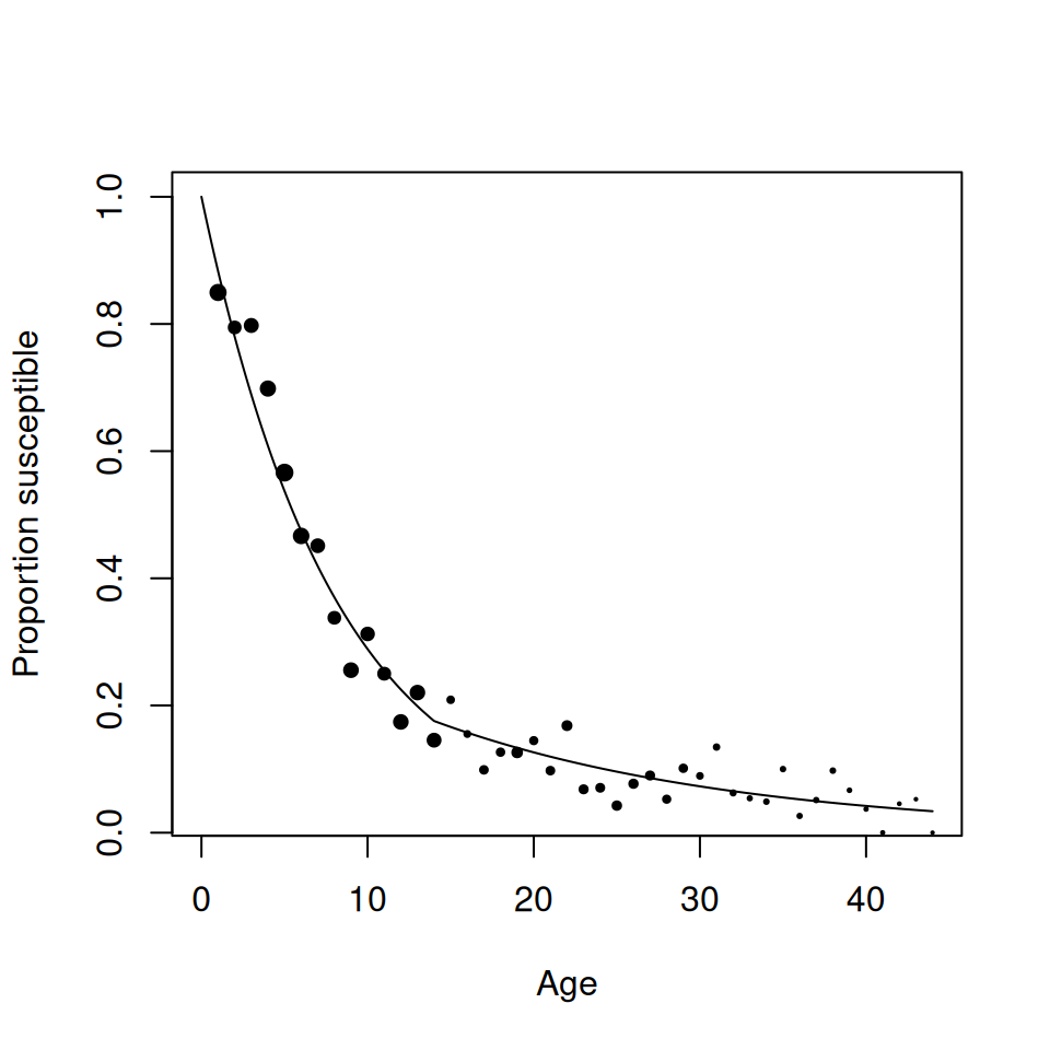

Figure 9.3: Predicted susceptible profile of two-group FOI model against data

Task

Can you suggest, and estimate, a model to improve the fit to the data? How can you compare the fit of the two models?

Solution

There is a suggestion from Figure 9.3 that infants, as well as adults, have a lower rate of infection than school age children. Such a “core-group” model will provide a closer fit to the serological age-profile.

## set up FOI mappings
three_groups <- rep(NA, max(rubella$Age))
three_groups[1:max(rubella$Age) < 5] <- 1
three_groups[1:max(rubella$Age) >= 5 & 1:max(rubella$Age) < 15] <- 2
three_groups[1:max(rubella$Age) >= 15] <- 3

## fit model
threegroup_mle <- optim(
    c(0.07, 0.07, 0.07),
    FOI_loglik,
    foi_key = three_groups,
    sero_data = rubella,
    control = list(fnscale = -1)
)
threegroup_mle

## $par
## [1] 0.10299635 0.14664689 0.04503626
## 
## $value
## [1] -105.7169
## 
## $counts
## function gradient 
##       88       NA 
## 
## $convergence
## [1] 0
## 
## $message
## NULL

## plot model fits
plot(
    ages, 
    piecewise_s(ages, threegroup_mle$par[three_groups]),
    type = 'l',
    xlab = "Age",
    ylab = "Proportion susceptible"
)
points(rubella$Age, rubella$p_s, pch = 19, cex = size^0.75)

The log-likelihood of -106 compared to -111 for the two group model, provides evidence that the three-group model better explains the data even allowing for any penalties we might chose to impose due to the additional parameter (e.g. AIC).

9.1.1 Bayesian estimation

We can also estimate the posterior distributions for the two force-of-infections within a Bayesian framework using MCMC. Here we introduce and use one of the standard MCMC libraries in R (MCMCpack) that implements a generic MCMC method.

Show: A note on priors

The function MCMCmetrop1R() provided in the MCMCpack library takes a function that returns the un-normalised log-posterior density, that is: \[\begin{equation} \log\left[f\left(\mathbf{y} \mid \boldsymbol{\theta}\right)\right] + \log\left[f\left(\boldsymbol{\theta}\right)\right]. \tag{9.3} \end{equation}\] We implement this using the FOI_loglik() function defined earlier. If we only export the log-likelihood from this function, then this is equivalent to putting completely flat (so-called improper) priors on the parameters. A subtlety here is that FOI_loglik() actually returns NA if any of the parameters are negative, meaning that in fact we are putting flat priors on \(\lambda_1\) and \(\lambda_2\) that are constrained in the region \((0, \infty)\). This is important since we know that rates can’t be negative.

If we want to use more structured prior distributions, then we would have to amend FOI_loglik() to return (9.3) with the correct prior densities built-in.

Important: you must know what priors you are using, since they are an integral part of a Bayesian analysis.

## load library
library(MCMCpack) 

## fit model
twogroup_post <- MCMCmetrop1R(
    FOI_loglik,                     ## log-likelihood 
    theta.init = twogroup_mle$par,  ## initial values
    mcmc = 10000,                   ## number of iterations
    burnin = 500,                   ## burn-in
    tune = 1,                       ## proposal parameter
    verbose = 500,                  ## print progress every 500 it
    logfun = TRUE,                  ## return log-density
    foi_key = two_groups,           ## foi key
    sero_data = rubella             ## data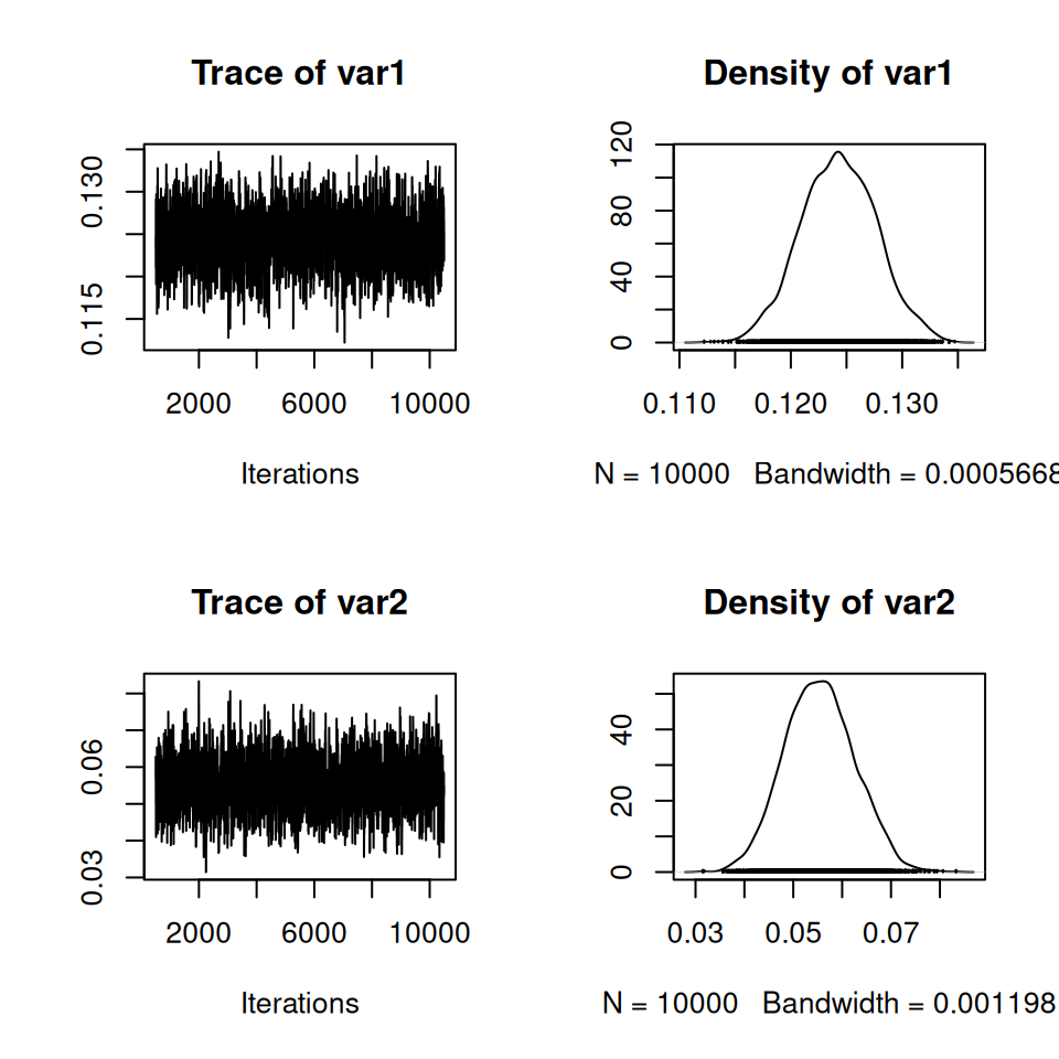
)

Task

Check the convergence of the MCMC and comment on the weight of evidence that the force-of-infection for rubella is different in the two age groups.

Show: Hint

Plotting the fitted model object will give the trace plots, and summarising the model object gives useful summary measures.

Solution

To check the chains we can simply plot the two_group_post object:

plot(twogroup_post)

summary(twogroup_post)

## 
## Iterations = 501:10500
## Thinning interval = 1 
## Number of chains = 1 
## Sample size per chain = 10000 
## 
## 1. Empirical mean and standard deviation for each variable,
##    plus standard error of the mean:
## 
##         Mean       SD  Naive SE Time-series SE
## [1,] 0.12432 0.003374 3.374e-05      0.0001069
## [2,] 0.05539 0.007129 7.129e-05      0.0002193
## 
## 2. Quantiles for each variable:
## 
##         2.5%    25%     50%     75%   97.5%
## var1 0.11765 0.1220 0.12432 0.12667 0.13112
## var2 0.04191 0.0504 0.05521 0.06025 0.06946

Here the chains look well mixed and the algorithm seems to have converged (ideally we would want to run multiple chains). The 95% credible intervals for the two force of infection parameters are non-overlapping with a risk of infection for school age-children almost twice that of adults.

9.2 Next-generation matrix approaches

If the force-of-infection was independent of age we could estimate \(R_0\) straightforwardly as the ratio of the force-of-infection and life expectancy. However, when the force-of-infection varies with age we need to first use the force-of-infection to calculate the transmission parameters within and between each age-group. Here we work through through the traditional method for achieving this where social contact data is not available and assumptions must be made about Who Acquires Infection from Whom (WAIFW).

We can derive an equation that links the force-of-infection and the elements of the next generation matrix \(k_{ij}\). (The details of the derivation are a little messy and will be omitted here, see Anderson and May (1991); Hens et al. (2012) for details.)

\[\begin{equation} \begin{pmatrix} \beta_{11} & \beta_{12}\\ \beta_{21} & \beta_{22} \end{pmatrix} \begin{pmatrix} \psi_1 \\ \psi_2 \end{pmatrix} = \begin{pmatrix} \lambda_1 \\ \lambda_2 \end{pmatrix} \tag{9.4} \end{equation}\]

\(\mathbf{\psi}\) is a function derived from the force-of-infection that, loosely, corresponds to the average proportion of individuals infectious within each age group at any time. The function Psi(lambda, age_widths, TI, u) defined below returns the vector \(\mathbf{\psi}\) for a specified force-of-infection lambda, for coarse age groups of widths age_widths, and infectious period of length TI, and the mortality rate for each age group u.

Psi <- function(lambda, age_widths, u, TI) {
    
    ## set up auxiliary vectors
    psi <- numeric(length(lambda))
    Psi <- numeric(length(lambda))
    
    ## calculate elements of psi-vector
    psi <- lambda * age_widths
    psi <- cumsum(psi)
    Psi[1] <- 1 - exp(-psi[1])
    for(a in 2:length(lambda)) {
        Psi[a] <- exp(-psi[a - 1]) - exp(-psi[a])
    }
    
    ## return psi-vector
    return((u / (1 / TI)) * Psi)
}

Equation (9.4) defines two simultaneous equations for two known values: \(\left(\lambda_1, \lambda_2\right)\).

We can only proceed to solve these equations by restricting the values of \(k_{ij}\) to the number of estimated forces-of-infection. Different assumptions about the structure of this matrix correspond to very different estimates of \(R_0\). Greenhalgh and Dietz (1994) demonstrated that the feasible lower bound on \(R_0\) for these data corresponds to the situation where infants are responsible for all transmission within the population: \[\begin{equation} \mbox{infant} = \begin{pmatrix} k_1 & 0\\ k_2 & 0 \end{pmatrix}. \end{equation}\] The upper bound corresponds to the diagonal matrix where mixing occurs purely within your own age group: \[\begin{equation} \mbox{diagonal} = \begin{pmatrix} k_1 & 0\\ 0 & k_2 \end{pmatrix}. \end{equation}\]

Task

By substituting these matrices into equation (9.4) and carrying out the matrix multiplication, find expressions for \(k_1\) and \(k_2\) in terms of \(\left(\lambda_1, \lambda_2, \psi_1, \psi_2\right)\).

Solution

For the ‘infant’ matrix: \[ k_1 = \frac{\lambda_1}{\psi_1} \qquad \mbox{and} \qquad k_2 = \frac{\lambda_2}{\psi_1}. \] For the ‘diagonal’ matrix: \[ k_1 = \frac{\lambda_1}{\psi_1} \qquad \mbox{and} \qquad k_2 = \frac{\lambda_2}{\psi_2}. \]

Task

Use your new expressions to calculate the values of \(k\) for the infant mixing and assortative mixing assumptions, and the corresponding lower and upper bounds for \(R_0\). Use the maximum likelihood estimates of \(\lambda_1\) and \(\lambda_2\). Assume that the mortality rate \(u = 20 / 1000\) and that \(T_I = 5 / 365\). Assume the total population size is \(n = 1\).

Show: Hint

You will need to use the max(), eigen() and matrix() functions. Remember that here the NGM is \(T_I \boldsymbol{\beta}\mathbf{n}\), where \(\mathbf{n}\) is the proportion of the population in each age-class, and \(T_I\) is the average length of the infectious period.

Solution

## set up mortality rate and infectious period
u <- 20 / 1000
TI <- 5 / 365

## calculate psi
psi <- Psi(twogroup_mle$par, age_widths = c(15, 30), u, TI)

## proportion of population in the two age groups (exponential 
## age-distribution)
n <- c((1 - exp(-15 * u)), exp(-15 * u))

## infant mixing MLE
k1 <- twogroup_mle$par[1] / psi[1]
k2 <- twogroup_mle$par[2] / psi[1]
max(TI * eigen(matrix(c(k1, k2, 0, 0), 2, 2) * n)$values)

## [1] 1.905538

## diagonal mixing MLE
k1 <- twogroup_mle$par[1] / psi[1]
k2 <- twogroup_mle$par[2] / psi[2]
max(TI * eigen(matrix(c(k1, 0, 0, k2), 2, 2) * n)$values)

## [1] 16.25391

Task

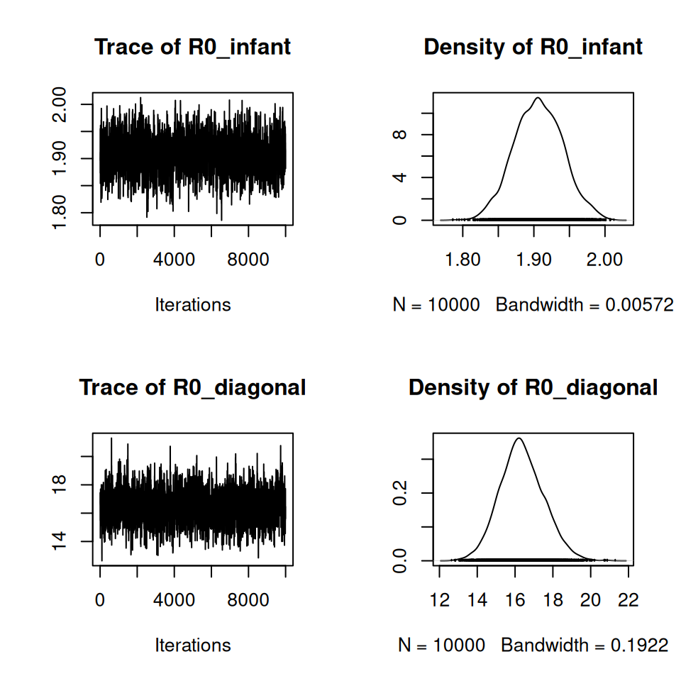
Calculate the posterior distributions for \(R_0\) for the two-group model under the same conditions as the previous task. Plot the posterior densities.

Show: Hint

Convert the twogroups_post into a matrix using as.matrix(), and then either loop over the samples, or use apply() to generate posterior samples for \(\psi_1\) and \(\psi_2\). These can then be converted into posterior samples for \(k_1\) and \(k_2\) and correspondingly into posterior samples for \(R_0\). as.mcmc() can be used to turn matrix objects into mcmc objects for ease of plotting and summarisation (or just work with the matrix objects directly).

Solution

## calculate psi for each posterior sample
psi <- t(apply(as.matrix(twogroup_post), 1, function(x, u, TI) {
        Psi(x, age_widths = c(15, 30), u, TI)
    }, u = u, TI = TI))

## infant mixing posterior samples
k1 <- twogroup_post[, 1] / psi[, 1]
k2 <- twogroup_post[, 2] / psi[, 1]
R0_infant <- apply(cbind(k1, k2), 1, function(k, n, TI) {
        max(TI * eigen(matrix(c(k[1], k[2], 0, 0), 2, 2) * n)$values)
    }, n = n, TI = TI)

## diagonal mixing MLE
k1 <- twogroup_post[, 1] / psi[, 1]
k2 <- twogroup_post[, 2] / psi[, 2]
R0_diagonal <- apply(cbind(k1, k2), 1, function(k, n, TI) {
        max(TI * eigen(matrix(c(k[1], 0, 0, k[2]), 2, 2) * n)$values)
    }, n = n, TI = TI)

## plot and summarise
R0 <- as.mcmc(cbind(R0_infant, R0_diagonal))
plot(R0)

summary(R0)

## 
## Iterations = 1:10000
## Thinning interval = 1 
## Number of chains = 1 
## Sample size per chain = 10000 
## 
## 1. Empirical mean and standard deviation for each variable,
##    plus standard error of the mean:
## 
##               Mean      SD  Naive SE Time-series SE
## R0_infant    1.907 0.03405 0.0003405       0.001079
## R0_diagonal 16.360 1.16207 0.0116207       0.035975
## 
## 2. Quantiles for each variable:
## 
##              2.5%    25%    50%   75%  97.5%
## R0_infant    1.84  1.883  1.906  1.93  1.976
## R0_diagonal 14.18 15.577 16.311 17.11 18.735

9.3 Estimating the next generation matrix from rubella serology

For human infectious diseases at least, the POLYMOD social contact data has revolutionised how we interpret serological data. In this section we estimate the next generation matrix for rubella using the POLYMOD mixing data. We also introduce a more modern, and convenient, method where we directly estimate the next generation matrix from age-stratified serological data.

For a given next generation matrix K we can calculate the resulting force-of-infection using: \[\begin{equation} \lambda_i = \sum_{j} k_{ij}\left[P_s\left(a_{i + 1}\right) - P_s\left(a_i\right)\right] \tag{9.5} \end{equation}\] Although we cannot write down a closed form solution for \(K_{ij}\), for any given next generation matrix \(\mathbf{K}\), we can iteratively solve equations (9.2) and (9.5) to obtain the susceptibility curve \(P_s(a)\) and force-of-infection \(\lambda_i\) that correspond to particular values of \(\mathbf{K}\). By exploring different values (and forms) of \(\mathbf{K}\) we can then estimate what next generation matrix is most consistent with a given susceptibility curve.

This procedure is straightforward, but a bit fiddly, so once again we have provided you with helper functions below to do this, adapted from the book by Hens et al. (2012).

NextGen_foi(K) returns the age-stratified force-of-infection corresponding to a specified next generation matrix K (Equation (9.5) above). The number of age groups is taken from the dimensions (number of rows/columns) of K.

NextGen_loglik(x, matrixfunction, sero_data) is analogous to FOI_loglik() and returns the likelihood of observing a given number of positive/negative samples for each age-group and a specified next generation matrix with parameters x and structure defined by a user specified function matrixfunction().

Note that instead of estimating the scaling parameter \(y = e^x\) directly, we estimate \(x = e^y\). This parameter transformation doesn’t change our basic assumption that transmission is directly proportional to the reported POLYMOD contacts, but improves the numerical accuracy of our estimation. Such tricks often improve the convergence of numerical procedures, especially MCMC methods, but the appropriate choice can be somewhat of a black art.

By writing NextGen_loglik() to depend on a function as well as a set of parameters we can easily fit alternative models that assume different patterns of mixing in the population. For example we can specify a homogeneous mixing model by the following function:

## function that returns a homogeneous mixing next 
## generation matrix with all elements equal to x
HomogeneousMatrix <- function(x) { 
    mat <- matrix(x, 86, 86) 
    return(mat)
}

where we assume there are 86 age cohorts in the population (for consistency with POLYMOD matrix).

The helper functions are defined below:

## calculate force of infection for a given next generation matrix K
##
## annual age cohorts are assumed with maximum assumed age given by
## dimensions of K
##
## Arguments:
## K - Next Generation Matrix
NextGen_foi <- function(K) {
    ## set up age-class widths
    widths <- rep(1, nrow(K))
    ## number of age classes
    num_class <- nrow(K)
    ## piecewise FOI by age-class
    lambda <- numeric(num_class)
    ## susceptible fraction at END of age class
    s <- rev(sort(runif(num_class)))
    oldlambda <- lambda
    tolerance <- 1
    iterations <- 1
    while ((tolerance > 1e-10) & (iterations < 2000)) {
        oldlambda <- lambda
        for(i in 1:num_class) {
            lambda[i] <- (K[i, 1] * (1 - s[1]) + 
                sum(K[i, 2:num_class] * 
                (s[1:(num_class - 1)] - s[2:num_class])))
        }
        s[1] <- exp(-lambda[1] * widths[1])
        for(i in 2:(num_class)) {
            s[i] <- s[i - 1] * exp(-lambda[i] * widths[i])
        }
        tolerance <- sum((lambda - oldlambda)^2)
        iterations <- iterations + 1
    }
    return(lambda)
}

## calculate (Binomial) likelihood of observing given number of
## positive/negative samples 
## (provided in table sero_data) for each age group and specified 
## next generation matrix K = matrixfunction(x) 
## 
## Arguments:
## x: vector of unique force of infection values
## foi_key: pattern vector of length equal to the maximum assumed age
##    in population (or data set) that specifies which unique value of 
##    x corresponds to each annual cohort in population.
## sero_data: data frame with columns
## sero_data$Pos: positive samples
## sero_data$Neg: negative samples
NextGen_loglik <- function(x, matrixfunction, sero_data) {
    
    ## set up auxiiary vectors
    x <- exp(x)
    K <- matrixfunction(x)
    breaks <- 0:nrow(K)
    widths <- rep(1, nrow(K))
    
    if(any(x <= 0)) {
        ## if any rates < 0 then 
        ## return log-likelihood = -Inf
        return(-Inf)
    } else {
        ## calculate fois
        lambda <- NextGen_foi(K)
        
        ## calculate log-likelihoods
        loglik <- 0.0
        for(i in 1:nrow(sero_data)) {
            ## which age class does observation lie in 
            age_class <- max(which(sero_data$Age[i] > breaks))
            ## proportion of susceptibles at beginning of age class
            sg <- piecewise_s(breaks[age_class], lambda)
            loglik <- loglik + dbinom(
                sero_data$Pos[i],
                sero_data$Pos[i] + sero_data$Neg[i],
                prob = 1 - sg * exp(-lambda[age_class] * 
                    (sero_data$Age[i] - breaks[age_class])),
                log = TRUE
            )
        }
        ## return log-likelihood
        return(loglik)
    }
}

Show: The optimise() function

We used optim() earlier to optimise a function with respect to multiple parameters. If you want to optimise a function with respect to a single parameter, then we use optimise() instead. This works in a similar way, but has slightly different arguments. Most notably, rather than giving initial values for the parameter, we instead define an upper and lower bound over which to search for a maximum or minimum.

Arguments for optimise() can be found from the help file in the usual way e.g. ?optimise. The key ones here are:

• f: a function to be minimised (or maximised), with first argument the vector of parameters over which optimisation is to take place. It should return a scalar result. Here we pass it the NextGen_loglik() function we defined above.
• interval: a vector containing the end-points of the interval to be searched for the minimum (or maximum).
• ...: additional arguments required for NextGen_loglik() can be passed to optimise(); here we pass matrixfunction and sero_data arguments.
• maximum: a logical defining whether we maximise (TRUE) or minimise (FALSE).

Please see the help file for more details.

We can now obtain the maximum-likelihood estimate for the homogeneous mixing matrix by optimising the value of NextGen_loglik():

homogeneous_mle <- optimise(
    NextGen_loglik,                       ## function to optimise
    log(c(0.01, 1)),                      ## upper and lower bound
    matrixfunction = HomogeneousMatrix,   ## pass matrixfunction to NextGen_loglik
    sero_data = rubella,                  ## pass sero_data to NextGen_loglik
    maximum = TRUE                        ## maximise the function
)
homogeneous_mle

## $maximum
## [1] -2.209086
## 
## $objective
## [1] -135.6114

Then to calculate the force-of-infection corresponding to our maximum likelihood fit:

homogeneous_foi <- NextGen_foi(
    HomogeneousMatrix(exp(homogeneous_mle$maximum))
)

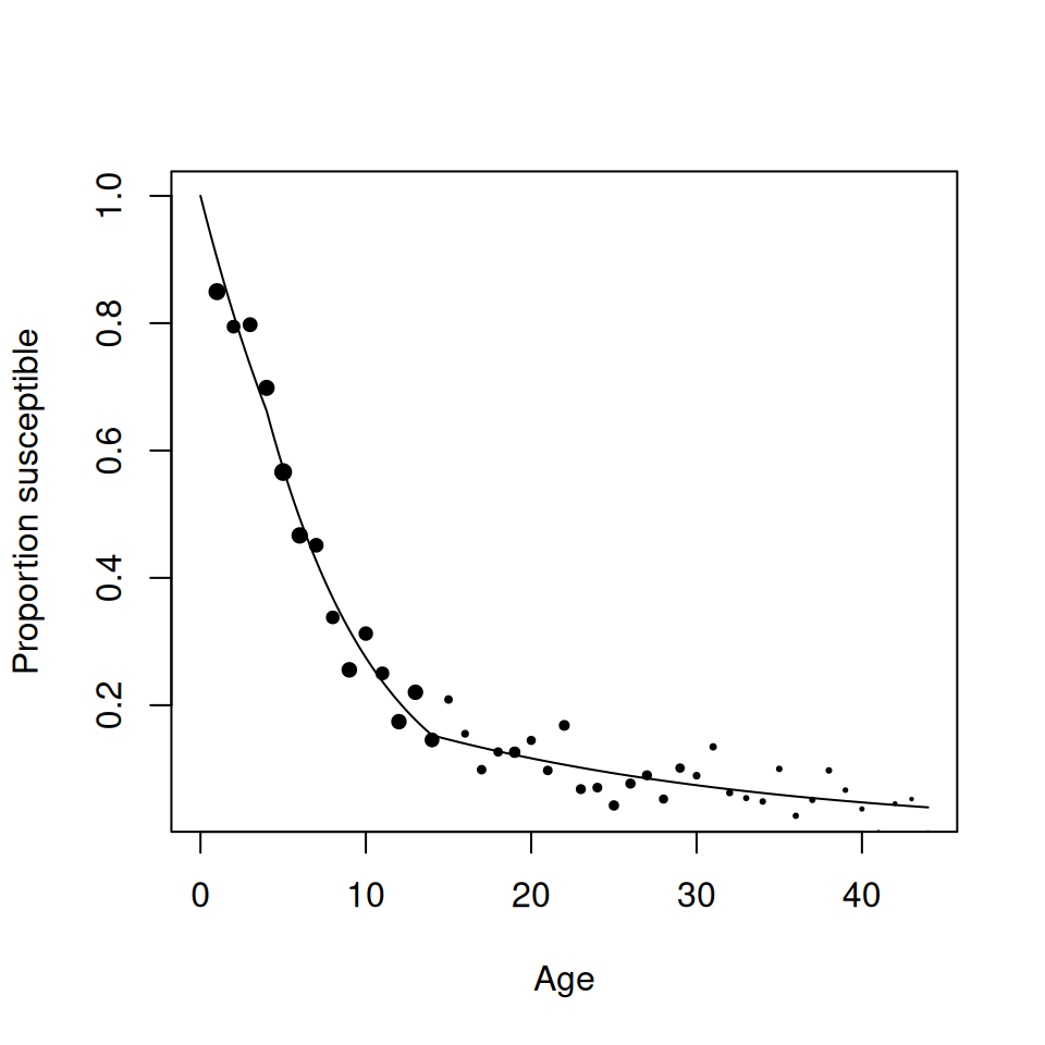
You can check the fit of the model by using the piecewise_s() function to predict the proportion positive for each age group and plot against the original data:

plot(rubella$Age, rubella$p_s, pch = 19, cex = size^0.75)
lines(
    seq(0.5, 75, 1), 
    piecewise_s(
        seq(0.5, 75, 1), 
        homogeneous_foi
    ),
    lwd = 2
)

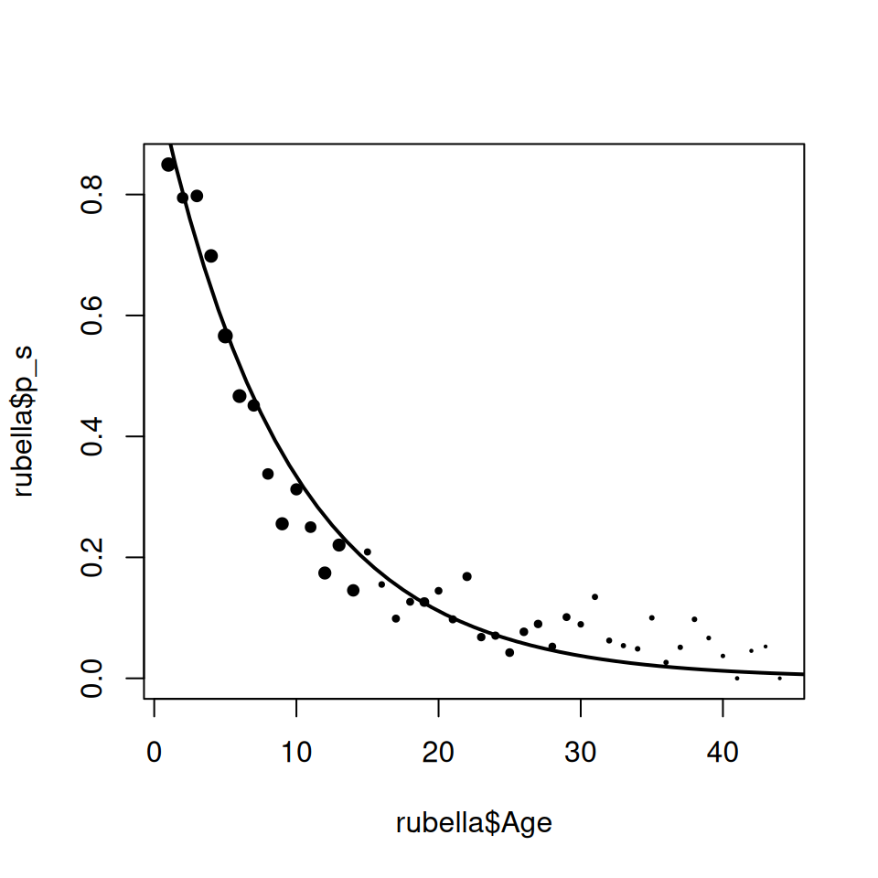
The overall fit is actually pretty good. However if we look closely the model does systematically overestimate the proportion infected in 10–20 year olds and underestimates in the 20–44 age groups, as we would expect from our analysis in the earlier section.

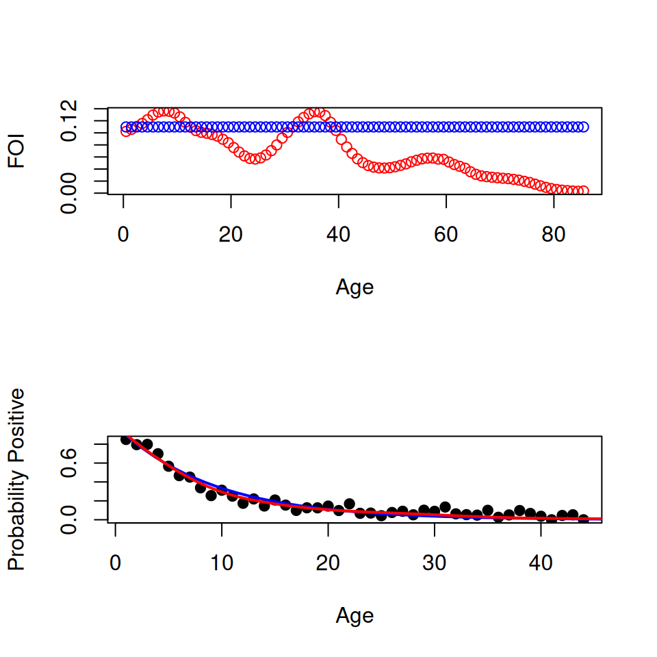
We could generalise our mixing matrix to include additional parameters to describe this heterogeneity as before. Or we can test whether social contact patterns provide a better description of the observed force-of-infection. Here we assume that infectious contacts are distributed proportionally to a POLYMOD mixing matrix.

Download the POLYMOD.csv file to your working directory and load into R:

## load (smoothed symmetrical) POLYMOD matrix 
POLYMOD <- as.matrix(read.csv("POLYMOD.csv", header = FALSE))

Now we write a function called POLYMODMatrix() that takes a single parameter x and returns a scaled version of the POLYMOD matrix (\(M_{ij}\)):

## generates a scaled POLYMODMatrix with transmission 
## parameter defined by x 
POLYMODMatrix <- function(x) { 
    return(x * POLYMOD)
}

Task

Follow the same steps as before to find the maximum likelihood estimate of the next generation matrix for the POLYMOD assumption and create a plot comparing the estimated force-of-infection and model fit for both models.

Solution

POLYMOD_mle <- optimise(
    NextGen_loglik,
    c(1, 15),
    matrixfunction = POLYMODMatrix,
    sero_data = rubella,
    maximum = TRUE 
)
POLYMOD_foi = NextGen_foi(POLYMODMatrix(exp(POLYMOD_mle$maximum)))
par(mfrow = c(2, 1))
plot(
    seq(0.5, 86, 1), 
    POLYMOD_foi, 
    type = 'b', 
    xlab = 'Age', 
    ylab = 'FOI', 
    col = 'red'
)
lines(seq(0.5, 86, 1), homogeneous_foi, type = 'b', col = 'blue')
plot(
    rubella$Age,
    rubella$p_s,
    pch = 19,
    xlab = 'Age',
    ylab = 'Probability Positive'
)
lines(
    seq(0.5, 86, 1), 
    piecewise_s(seq(0.5, 86, 1), homogeneous_foi), 
    lwd = 2, 
    col = 'blue'
)
lines(
    seq(0.5, 86, 1),
    piecewise_s(seq(0.5, 86, 1), POLYMOD_foi),
    lwd = 2,
    col = 'red'
)
par(mfrow = c(1, 1))

Finally, calculate the value of \(R_0\) for the two mixing assumptions:

max(Re(eigen(HomogeneousMatrix(exp(homogeneous_mle$maximum)))$values))   

## [1] 9.442879

max(Re(eigen(POLYMODMatrix(exp(POLYMOD_mle$maximum)))$values)) 

## [1] 7.777768

Question

Does the POLYMOD mixing provide a better fit to the rubella serological data?

Answer

The homogeneous mixing model has a maximum (log) likelihood value of -136, compared to -117 for the POLYMOD model. On this basis, and from visual inspection of the fit, the POLYMOD mixing model is better supported by the data, although we might want to produce measures such as AIC that penalise for model complexity before drawing firm conclusions.

Question

How do the predictions of the POLYMOD mixing model differ from homogeneous mixing?

Answer

The POLYMOD mixing assumption estimates a lower basic reproductive ratio than homogeneous mixing, implying that a lower level of vaccination coverage would be necessary to eliminate disease than might be expected under homogeneous mixing.

However, more importantly the POLYMOD model predicts a very different pattern of transmission within the population. The POLYMOD mixing matrix generates two equal peaks in the force of infection that are both higher than the homogeneous mixing estimate. The second peak in young adults is of particular concern for rubella where the disease itself is of less concern than so-called congenital rubella syndrome (CRS)—where infection of pregnant women leads to severe problems for unborn children. Pre-vaccination, with a mean age of infection of ~10 years this second group was relatively unimportant as few susceptible individuals ‘survived’ to that age. But it may become more important after the introduction of vaccination which is likely to increase the mean age of infection into this second core-group. This is the motivation for supplemental vaccination campaigns in teenage girls—i.e. not to reduce the rate of transmission in the community but to directly protect against CRS. The magnitude of this, so-called perverse effect of vaccination, would be greatly underestimated by a (incorrect) assumption of homogeneous mixing.

References

Anderson, R. M., and R. M. May. 1991. Infectious Diseases of Humans. Oxford University Press.

Greenhalgh, David, and Klaus Dietz. 1994. “Some Bounds on Estimates for Reproductive Ratios Derived from the Age-Specific Force of Infection.” Mathematical Biosciences 124 (1): 9–57. https://doi.org/10.1016/0025-5564(94)90023-X.

Hens, Niel, Ziv Shkedy, Marc Aerts, Christel Faes, Pierre Van Damme, and Philippe Beutels. 2012. Modeling Infectious Disease Parameters Based on Serological and Social Contact Data. Springer. https://doi.org/10.1007/978-1-4614-4072-7.